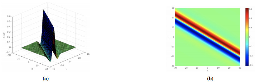
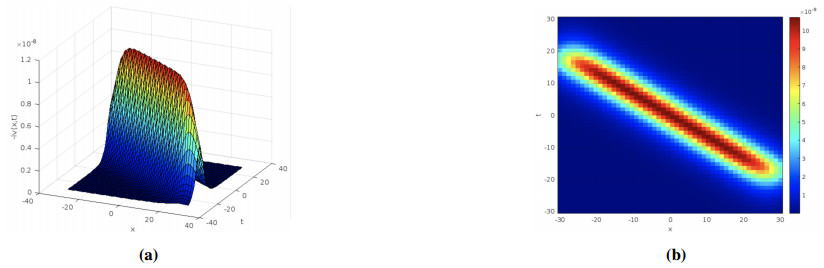
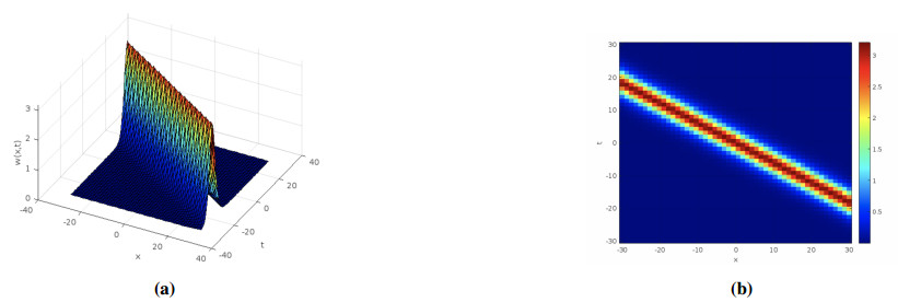
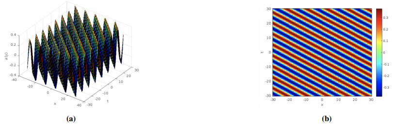
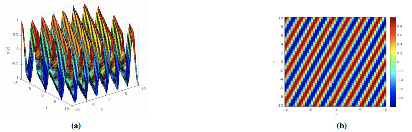
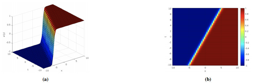
In this paper, we study an integrable system with the self-consistent potentials called the Nurshuak-Tolkynay-Myrzakulov (NTM) system. This system is of great importance in the theory of integrable nonlinear equations, since this system describes the dynamics of nonlinear wave processes in various fields of physics, such as hydrodynamics, optics, quantum mechanics, and plasma dynamics. Various integrable reductions of this system are also given and their Lax pairs are found. It is shown that the NTM system, being integrable, has some deep geometric roots, and that its geometric interpretation can lead to an understanding of more complex geometric structures. Thus, it is shown that the NTM system describes the dynamics of waves and allows us to understand how those waves interact with the geometry of space, which is an important aspect of many physical processes. Solitonic solutions of the NTM system are found. These solutions exhibit various signs of the periodicity, exponentiality, and rationality of soliton structures, including the elliptic Jacobi function. The results are visualized using three-dimentional (3D) and contour plots to clearly illustrate the response of the behavior to momentum propagation and to find appropriate values for the system's parameters. This visualization provides valuable insights into the characteristics and dynamics of the soliton solutions obtained from the integrable NTM equation.
Citation: Gulgassyl Nugmanova, Aidana Azhikhan, Ratbay Myrzakulov, Akbota Myrzakul. Nurshuak-Tolkynay-Myrzakulov system: integrability, geometry and solutions[J]. AIMS Mathematics, 2025, 10(6): 14167-14182. doi: 10.3934/math.2025638
In this paper, we study an integrable system with the self-consistent potentials called the Nurshuak-Tolkynay-Myrzakulov (NTM) system. This system is of great importance in the theory of integrable nonlinear equations, since this system describes the dynamics of nonlinear wave processes in various fields of physics, such as hydrodynamics, optics, quantum mechanics, and plasma dynamics. Various integrable reductions of this system are also given and their Lax pairs are found. It is shown that the NTM system, being integrable, has some deep geometric roots, and that its geometric interpretation can lead to an understanding of more complex geometric structures. Thus, it is shown that the NTM system describes the dynamics of waves and allows us to understand how those waves interact with the geometry of space, which is an important aspect of many physical processes. Solitonic solutions of the NTM system are found. These solutions exhibit various signs of the periodicity, exponentiality, and rationality of soliton structures, including the elliptic Jacobi function. The results are visualized using three-dimentional (3D) and contour plots to clearly illustrate the response of the behavior to momentum propagation and to find appropriate values for the system's parameters. This visualization provides valuable insights into the characteristics and dynamics of the soliton solutions obtained from the integrable NTM equation.

| [1] |
M. J. Ablowitz, D. J. Kaup, A. C. Newell, H. Segur, Method for solving the Sine-Gordon equation, Phys. Rev. Lett., 30 (1973), 1262. https://doi.org/10.1103/PhysRevLett.30.1262 doi: 10.1103/PhysRevLett.30.1262

|
| [2] |
G. L. Lamb, Solitons on moving space curves, J. Math. Phys., 18 (1977), 1654–1661. https://doi.org/10.1063/1.523453 doi: 10.1063/1.523453
|
| [3] | M. J. Ablowitz, H. Segur, Solitons and the inverse scattering transform, Philadelphia: Society for Industrial and Applied Mathematics, 1981. https://doi.org/10.1137/1.9781611970883 |
| [4] |
Q. Ding, J. Inoguchi, Schr${\ddot o}$dinger flows, binormal motion of curves and the second AKNS hierarchies, Chaos Soliton. Fract., 21 (2004), 669–677. https://doi.org/10.1016/j.chaos.2003.12.092 doi: 10.1016/j.chaos.2003.12.092
|
| [5] | C. Rogers, W. Shief, Bäcklund and Darboux transformations: geometry and modern applications in soliton theory, Cambridge: Cambridge University Press, 2002. https://doi.org/10.1017/CBO9780511606359 |
| [6] | X. Gao, Open-ocean shallow-water dynamics via a (2+1)-dimensional generalized variable-coefficient Hirota-Satsuma-Ito system: oceanic auto-Bäcklund transformation and oceanic solitons, China Ocean Eng., in press. https://doi.org/10.1007/s13344-025-0057-y |
| [7] |
X. Gao, In an ocean or a river: bilinear auto-Bäcklund transformations and similarity reductions on an extended time-dependent (3+1)-dimensional shallow water wave equation, China Ocean Eng., 39 (2025), 160–165. https://doi.org/10.1007/s13344-025-0012-y doi: 10.1007/s13344-025-0012-y
|
| [8] |
X. Gao, Hetero-Bäcklund transformation, bilinear forms and multi-solitons for a (2+1)-dimensional generalized modified dispersive water-wave system for the shallow water, Chinese J. Phys., 92 (2024), 1233–1239. https://doi.org/10.1016/j.cjph.2024.10.004 doi: 10.1016/j.cjph.2024.10.004
|
| [9] |
F. Arif, A. Jhangeer, F. Mahomed, F. Zaman, Lie group classification and conservation laws of a (2+1)-dimensional nonlinear damped Klein-Gordon Fock equation, Partial Differential Equations in Applied Mathematics, 12 (2024), 100962. https://doi.org/10.1016/j.padiff.2024.100962 doi: 10.1016/j.padiff.2024.100962
|
| [10] |
A. Jhangeer, H. Ehsan, M. Riaz, A. Talafha, Impact of fractional and integer order derivatives on the (4+1)-dimensional fractional Davey-Stewartson-Kadomtsev-Petviashvili equation, Partial Differential Equations in Applied Mathematics, 12 (2024), 100966. https://doi.org/10.1016/j.padiff.2024.100966 doi: 10.1016/j.padiff.2024.100966
|
| [11] |
A. Jhangeer, K. U. Tariq, M. Nasir Ali, On some new travelling wave solutions and dynamical properties of the generalized Zakharov system, PLoS ONE, 19 (2024), e0306319. https://doi.org/10.1371/journal.pone.0306319 doi: 10.1371/journal.pone.0306319
|
| [12] |
M. Alqudah, M. AlMheidat, M. Alqarni, E. Mahmoud, S. Ahmad, Strange attractors, nonlinear dynamics and abundant novel soliton solutions of the Akbota equation in Heisenberg ferromagnets, Chaos Soliton. Fract., 189 (2024), 115659. https://doi.org/10.1016/j.chaos.2024.115659 doi: 10.1016/j.chaos.2024.115659
|
| [13] |
H. Kong, R. Guo, Dynamic behaviors of novel nonlinear wave solutions for the Akbota equation, Optik, 282 (2023), 170863. https://doi.org/10.1016/j.ijleo.2023.170863 doi: 10.1016/j.ijleo.2023.170863
|
| [14] |
B. Ceesay, M. Baber, N. Ahmed, M. Jawaz, J. Macías-Díaz, A. Gallegos, Harvesting mixed, homoclinic breather, M-shaped and other wave profiles of the Heisenberg Ferromagnet-type Akbota equation, Eur. J. Pure Appl. Math., 18 (2025), 5852. https://doi.org/10.29020/nybg.ejpam.v18i2.5851 doi: 10.29020/nybg.ejpam.v18i2.5851
|
| [15] |
Z. Sagidullayeva, G. Nugmanova, R. Myrzakulov, N. Serikbayev, Integrable Kuralay equations: geometry, solutions and generalizations, Symmetry, 14 (2022), 1374. https://doi.org/10.3390/sym14071374 doi: 10.3390/sym14071374
|
| [16] |
M. M. Tariq, M. B. Riaz, M. Aziz-ur-Rehman, Investigation of space-time dynamics of Akbota equation using Sardar sub-equation and Khater methods: unveiling bifurcation and chaotic structure, Int. J. Theor. Phys., 63 (2024), 210. https://doi.org/10.1007/s10773-024-05733-5 doi: 10.1007/s10773-024-05733-5
|
| [17] |
Z. Li, S. Zhao, Bifurcation, chaotic behavior and solitary wave solutions for the Akbota equation, AIMS Mathematics, 9 (2024), 22590–22601. https://doi.org/10.3934/math.20241100 doi: 10.3934/math.20241100
|
| [18] |
Q. Liu, Y. Zhao, H. Hao, Breather-breather interactions, rational and semi-rational solutions of an integrable spin system in optical fibers, Optik, 316 (2024), 172064. https://doi.org/10.1016/j.ijleo.2024.172064 doi: 10.1016/j.ijleo.2024.172064
|
| [19] |
H. Chen, Z. Zhou, Darboux transformation with a double spectral parameter for the Myrzakulov-I equation, Chinese Phys. Lett., 31 (2014), 120504. https://doi.org/10.1088/0256-307X/31/12/120504 doi: 10.1088/0256-307X/31/12/120504
|
| [20] |
S. C. Anco, R. Myrzakulov, Integrable generalizations of Schrödinger maps and Heisenberg spin models from Hamiltonian flows of curves and surfaces, J. Geom. Phys., 60 (2010), 1576–1603. https://doi.org/10.1016/j.geomphys.2010.05.013 doi: 10.1016/j.geomphys.2010.05.013
|
| [21] |
A. Myrzakul, G. Nugmanova, N. Serikbayev, R. Myrzakulov, Surfaces and curves induced by nonlinear Schrödinger-type equations and their spin systems, Symmetry, 13 (2021), 1827. https://doi.org/10.3390/sym13101827 doi: 10.3390/sym13101827
|
| [22] |
J. Muhammad, M. Bilal Riaz, U. Younas, N. Nasreen, A. Jhangeer, D. Lu, Extraction of optical wave structures to the coupled fractional system in magneto-optic waveguides, Arab Journal of Basic and Applied Sciences, 31 (2024), 242–254. https://doi.org/10.1080/25765299.2024.2337469 doi: 10.1080/25765299.2024.2337469
|
| [23] |
F. Ali, A. Jhangeer, M. Mudassar, A complete dynamical analysis of discrete electric lattice coupled with modified Zakharov-Kuznetsov equation, Partial Differential Equations in Applied Mathematics, 11 (2024), 100878. https://doi.org/10.1016/j.padiff.2024.100878 doi: 10.1016/j.padiff.2024.100878
|
| [24] |
M. Kousar, A. Jhangeer, M. Muddassar, Comprehensive analysis of noise behavior influenced by random effects in stochastic differential equations, Partial Differential Equations in Applied Mathematics, 12 (2024), 100997. https://doi.org/10.1016/j.padiff.2024.100997 doi: 10.1016/j.padiff.2024.100997
|
| [25] | M. Fecko, Differential geometry and Lie groups for physicists, Cambridge: Cambridge University Press, 2010. https://doi.org/10.1017/CBO9780511755590 |
| [26] |
R. Myrzakulov, G. Mamyrbekova, G. Nugmanova, K. Yesmakhanova, M. Lakshmanan, Integrable motion of curves in self-consistent potentials: relation to spin systems and soliton equations, Phys. Lett. A, 378 (2014), 2118–2123. https://doi.org/10.1016/j.physleta.2014.05.010 doi: 10.1016/j.physleta.2014.05.010
|
| [27] |
K. Farooq, E. Hussain, U. Younas, H. Mukalazi, T. M. Khalaf, A. Mutlib, et al., Exploring the wave's structures to the nonlinear coupled system arising in surface geometry, Sci. Rep., 15 (2025), 11624. https://doi.org/10.1038/s41598-024-84657-w doi: 10.1038/s41598-024-84657-w
|
| [28] |
B. Infal, A. Jhangeer, M. Muddassar, Dynamical patterns in stochastic $\rho^4$ equation: an analysis of quasi-periodic, bifurcation, chaotic behavior, Int. J. Geom. Methods M., 22 (2025), 2450320. https://doi.org/10.1142/S0219887824503201 doi: 10.1142/S0219887824503201
|
| [29] |
W. A. Faridi, M. A. Bakar, M. B. Riaz, Z. Myrzakulova, R. Myrzakulov, A. M. Mostafa, Exploring the optical soliton solutions of Heisenberg ferromagnet-type of Akbota equation arising in surface geometry by explicit approach, Opt. Quant. Electron., 56 (2024), 1046. https://doi.org/10.1007/s11082-024-06904-8 doi: 10.1007/s11082-024-06904-8
|
| [30] |
A. Myrzakul, R. Myrzakulov, Integrable geometric flows of interacting curves/surfaces, multilayer spin systems and the vector nonlinear Schrödinger equation, Int. J. Geom. Methods M., 14 (2017), 1750136. https://doi.org/10.1142/S0219887817501365 doi: 10.1142/S0219887817501365
|

Figures(7)

Gulgassyl Nugmanova, Aidana Azhikhan, Ratbay Myrzakulov, Akbota Myrzakul. Nurshuak-Tolkynay-Myrzakulov system: integrability, geometry and solutions[J]. AIMS Mathematics, 2025, 10(6): 14167-14182. doi: 10.3934/math.2025638


 DownLoad: