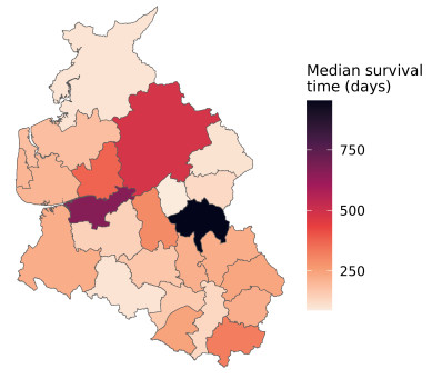
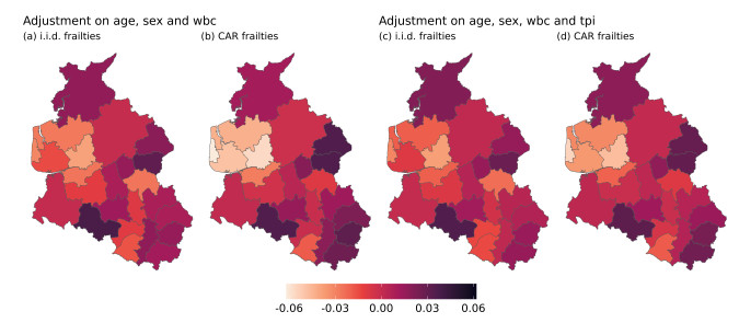
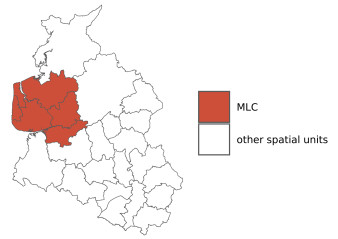
We propose a review of spatial scan statistics approaches in the context of survival data. After presenting the general principle of spatial scan statistics, we review the literature and find that few approaches exist. We distinguish between the first parametric approaches, based on a specific distribution model and therefore not very flexible, and a semi-parametric method. However, these approaches do not allow taking into account the spatial dependence frequently observed in the data. We then present a more recent approach allowing us to take them into account. Finally, we describe the adjustment of cluster detection on covariates before illustrating the methods on the detection of abnormal survival time clusters following the diagnosis of leukemia.
Citation: Camille Frévent. A review of spatial scan statistics for survival data[J]. AIMS Mathematics, 2025, 10(6): 14088-14101. doi: 10.3934/math.2025634
We propose a review of spatial scan statistics approaches in the context of survival data. After presenting the general principle of spatial scan statistics, we review the literature and find that few approaches exist. We distinguish between the first parametric approaches, based on a specific distribution model and therefore not very flexible, and a semi-parametric method. However, these approaches do not allow taking into account the spatial dependence frequently observed in the data. We then present a more recent approach allowing us to take them into account. Finally, we describe the adjustment of cluster detection on covariates before illustrating the methods on the detection of abnormal survival time clusters following the diagnosis of leukemia.

| [1] |
M. Kulldorff, N. Nagarwalla, Spatial disease clusters: detection and inference, Stat. Med., 14 (1995), 799–810. http://dx.doi.org/10.1002/sim.4780140809 doi: 10.1002/sim.4780140809

|
| [2] | M. Kulldorff, A spatial scan statistic, Commun. Stat.-Theory Methods, 26 (1997), 1481–1496. http://dx.doi.org/10.1080/03610929708831995 |
| [3] |
I. Jung, M. Kulldorff, A. C. Klassen, A spatial scan statistic for ordinal data, Stat. Med., 26 (2007), 1594–1607. http://dx.doi.org/10.1002/sim.2607 doi: 10.1002/sim.2607
|
| [4] |
M. Kulldorff, L. Huang, L. Pickle, L. Duczmal, An elliptic spatial scan statistic, Stat. Med., 25 (2006), 3929–3943. http://dx.doi.org/10.1002/sim.2490 doi: 10.1002/sim.2490
|
| [5] |
L. Cucala, C. Demattei, P. Lopes, A. Ribeiro, A spatial scan statistic for case event data based on connected components, Comput. Stat., 28 (2013), 357–369. http://dx.doi.org/10.1007/s00180-012-0304-6 doi: 10.1007/s00180-012-0304-6
|
| [6] |
T. Tango, K. Takahashi, A flexibly shaped spatial scan statistic for detecting clusters, Int. J. Health Geogr., 4 (2005), 11. http://dx.doi.org/10.1186/1476-072X-4-11 doi: 10.1186/1476-072X-4-11
|
| [7] |
P. S. Lin, Y. H. Kung, M. Clayton, Spatial scan statistics for detection of multiple clusters with arbitrary shapes, Biometrics, 72 (2016), 1226–1234. http://dx.doi.org/10.1111/biom.12509 doi: 10.1111/biom.12509
|
| [8] |
M. Kulldorff, L. Huang, K. Konty, A scan statistic for continuous data based on the normal probability model, Int. J. Health Geogr., 8 (2009), 58. http://dx.doi.org/10.1186/1476-072X-8-58 doi: 10.1186/1476-072X-8-58
|
| [9] |
L. Cucala, A distribution-free spatial scan statistic for marked point processes, Spat. Stat., 10 (2014), 117–125. http://dx.doi.org/10.1016/j.spasta.2014.03.004 doi: 10.1016/j.spasta.2014.03.004
|
| [10] |
I. Jung, H. J. Cho, A nonparametric spatial scan statistic for continuous data, Int. J. Health Geogr., 14 (2015), 30. http://dx.doi.org/10.1186/s12942-015-0024-6 doi: 10.1186/s12942-015-0024-6
|
| [11] |
L. Huang, M. Kulldorff, D. Gregorio, A spatial scan statistic for survival data, Biometrics, 63 (2007), 109–118. http://dx.doi.org/10.1111/j.1541-0420.2006.00661.x doi: 10.1111/j.1541-0420.2006.00661.x
|
| [12] |
V. Bhatt, N. Tiwari, A spatial scan statistic for survival data based on Weibull distribution, Stat. Med., 33 (2014), 1867–1876. http://dx.doi.org/10.1002/sim.6075 doi: 10.1002/sim.6075
|
| [13] |
V. Bhatt, N. Tiwari, A spatial scan statistic for survival data based on generalized life distribution, Commun. Stat.-Theory Methods, 45 (2016), 5730–5744. http://dx.doi.org/10.1080/03610926.2014.948207 doi: 10.1080/03610926.2014.948207
|
| [14] |
I. Usman, R. J. Rosychuk, A log-Weibull spatial scan statistic for time to event data, Int. J. Health Geogr., 17 (2018), 20. http://dx.doi.org/10.1186/s12942-018-0137-9 doi: 10.1186/s12942-018-0137-9
|
| [15] |
A. J. Cook, D. R. Gold, Y. Li, Spatial cluster detection for censored outcome data, Biometrics, 63 (2007), 540–549. http://dx.doi.org/10.1111/j.1541-0420.2006.00714.x doi: 10.1111/j.1541-0420.2006.00714.x
|
| [16] |
W. R. Tobler, A computer movie simulating urban growth in the Detroit region, Econ. Geogr., 46 (1970), 234–240. http://dx.doi.org/10.2307/143141 doi: 10.2307/143141
|
| [17] |
C. Frévent, M. S. Ahmed, S. Dabo-Niang, M. Genin, A shared‐frailty spatial scan statistic model for time‐to‐event data, Biometrical J., 66 (2024), e202300200. http://dx.doi.org/10.1002/bimj.202300200 doi: 10.1002/bimj.202300200
|
| [18] |
R. Henderson, S. Shimakura, D. Gorst, Modeling spatial variation in leukemia survival data, J. Am. Stat. Assoc., 97 (2002), 965–972. http://dx.doi.org/10.1198/016214502388618753 doi: 10.1198/016214502388618753
|
| [19] |
A. M. Abrams, K. Kleinman, M. Kulldorff, Gumbel based p-value approximations for spatial scan statistics, Int. J. Health Geogr., 9 (2010), 61. http://dx.doi.org/10.1186/1476-072X-9-61 doi: 10.1186/1476-072X-9-61
|
| [20] | Z. Zhang, R. Assunção, M. Kulldorff, Spatial scan statistics adjusted for multiple clusters, J. Probab. Stat., 2010. http://dx.doi.org/10.1155/2010/642379 |
Figures(3) / Tables(2)

Camille Frévent. A review of spatial scan statistics for survival data[J]. AIMS Mathematics, 2025, 10(6): 14088-14101. doi: 10.3934/math.2025634


 DownLoad: