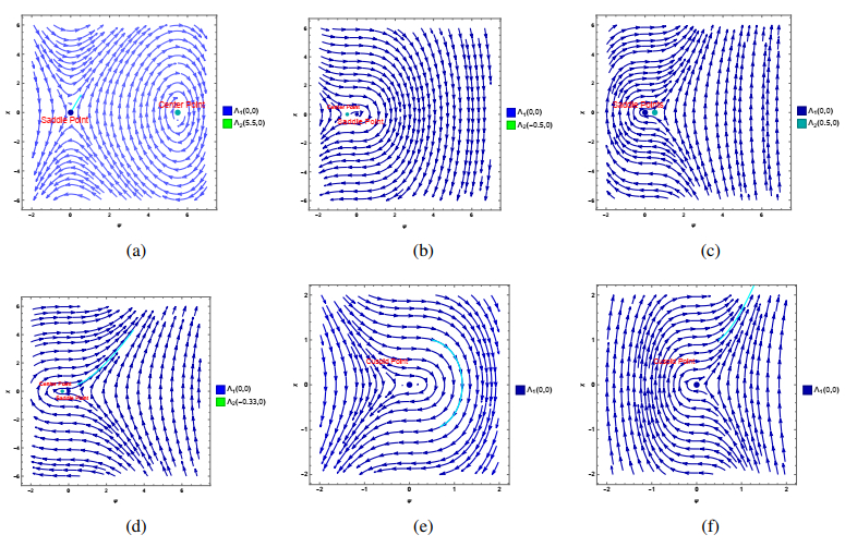
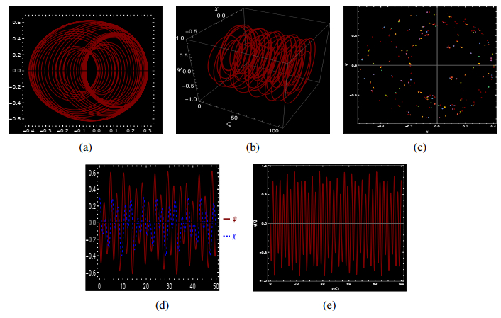
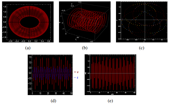
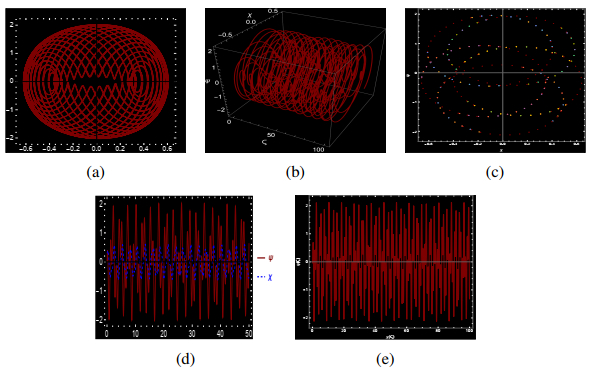
Loading [MathJax]/jax/output/SVG/jax.js
Research article Special Issues

Analytical solutions of the combined Kairat-Ⅱ-Ⅹ equation: a dynamical perspective on bifurcation, chaos, energy, and sensitivity

  • Received: 08 April 2025 Revised: 14 May 2025 Accepted: 27 May 2025 Published: 13 June 2025
  • MSC : 35C07, 35B32, 34Hxx, 49K40

  • In this study, we apply the (m+1Φ)-expansion and modified extended tanh function (METHF) methods to investigate the exact solutions of the new Kairat-Ⅱ-Ⅹ model. Using these methods, new exact solutions are derived for the proposed model. The hyperbolic, periodic, and singular forms of exact solutions are among those obtained. The propagating behaviors of wave solutions are depicted using three-dimensional (3D), contour, and two-dimensional (2D) surfaces, providing comprehensive visualizations of the wave dynamics. Physical meanings of the chosen solutions are determined through these simulations. Traveling wave solutions of nonlinear partial differential equations can be obtained using the techniques presented in this paper since they have been shown to be dependable, strong, and effective. Furthermore, the phase portrait has been thoroughly analyzed according to the equilibrium points, and various scenarios have been visualized using these portraits. With the use of time series graphs, Poincaré maps, and 3D and 2D plots, the impact of the perturbation term has been thoroughly investigated. The system's periodic, quasi-periodic, and chaotic structures are clearly illustrated by these depictions. The results enhance the understanding of the new Kairat-Ⅱ-Ⅹ equation's dynamic structure and how it applies to real-world events.

    Citation: Ulviye Demirbilek, Ali H. Tedjani, Aly R. Seadawy. Analytical solutions of the combined Kairat-Ⅱ-Ⅹ equation: a dynamical perspective on bifurcation, chaos, energy, and sensitivity[J]. AIMS Mathematics, 2025, 10(6): 13664-13691. doi: 10.3934/math.2025615

    Related Papers:

    [1] Mohammed Aldandani, Omar Naifar, Abdellatif Ben Makhlouf . Practical stability for nonlinear systems with generalized conformable derivative. AIMS Mathematics, 2023, 8(7): 15618-15632. doi: 10.3934/math.2023797
    [2] Yuanlin Ding . Existence and stability analysis of solutions for periodic conformable differential systems with non-instantaneous impulses. AIMS Mathematics, 2025, 10(2): 4040-4066. doi: 10.3934/math.2025188
    [3] Muhammad Bilal, Javed Iqbal, Ikram Ullah, Aditi Sharma, Hasim Khan, Sunil Kumar Sharma . Novel optical soliton solutions for the generalized integrable (2+1)- dimensional nonlinear Schrödinger system with conformable derivative. AIMS Mathematics, 2025, 10(5): 10943-10975. doi: 10.3934/math.2025497
    [4] Xuelian Jin . Exponential stability analysis and control design for nonlinear system with time-varying delay. AIMS Mathematics, 2021, 6(1): 102-113. doi: 10.3934/math.2021008
    [5] Aisha F. Fareed, Emad A. Mohamed, Mokhtar Aly, Mourad S. Semary . A novel numerical method for stochastic conformable fractional differential systems. AIMS Mathematics, 2025, 10(3): 7509-7525. doi: 10.3934/math.2025345
    [6] Awais Younus, Khizra Bukhsh, Manar A. Alqudah, Thabet Abdeljawad . Generalized exponential function and initial value problem for conformable dynamic equations. AIMS Mathematics, 2022, 7(7): 12050-12076. doi: 10.3934/math.2022670
    [7] Tan Zhang, Pianpian Yan . Asymmetric integral barrier function-based tracking control of constrained robots. AIMS Mathematics, 2024, 9(1): 319-339. doi: 10.3934/math.2024019
    [8] Noha M. Kamel, Hamdy M. Ahmed, Wafaa B. Rabie . Solitons unveilings and modulation instability analysis for sixth-order coupled nonlinear Schrödinger equations in fiber bragg gratings. AIMS Mathematics, 2025, 10(3): 6952-6980. doi: 10.3934/math.2025318
    [9] Narongrit Kaewbanjak, Watcharin Chartbupapan, Kamsing Nonlaopon, Kanit Mukdasai . The Lyapunov-Razumikhin theorem for the conformable fractional system with delay. AIMS Mathematics, 2022, 7(3): 4795-4802. doi: 10.3934/math.2022267
    [10] Erfeng Xu, Wenxing Xiao, Yonggang Chen . Local stabilization for a hyperchaotic finance system via time-delayed feedback based on discrete-time observations. AIMS Mathematics, 2023, 8(9): 20510-20529. doi: 10.3934/math.20231045
  • In this study, we apply the (m+1Φ)-expansion and modified extended tanh function (METHF) methods to investigate the exact solutions of the new Kairat-Ⅱ-Ⅹ model. Using these methods, new exact solutions are derived for the proposed model. The hyperbolic, periodic, and singular forms of exact solutions are among those obtained. The propagating behaviors of wave solutions are depicted using three-dimensional (3D), contour, and two-dimensional (2D) surfaces, providing comprehensive visualizations of the wave dynamics. Physical meanings of the chosen solutions are determined through these simulations. Traveling wave solutions of nonlinear partial differential equations can be obtained using the techniques presented in this paper since they have been shown to be dependable, strong, and effective. Furthermore, the phase portrait has been thoroughly analyzed according to the equilibrium points, and various scenarios have been visualized using these portraits. With the use of time series graphs, Poincaré maps, and 3D and 2D plots, the impact of the perturbation term has been thoroughly investigated. The system's periodic, quasi-periodic, and chaotic structures are clearly illustrated by these depictions. The results enhance the understanding of the new Kairat-Ⅱ-Ⅹ equation's dynamic structure and how it applies to real-world events.


    The differential equations of some problems are defined on infinite intervals of some engineering problems. Because of the infinite of calculation interval, how to calculate the upper boundary value problem of infinite interval becomes an important research subject for many numerical analysts.

    Semi-infinite domain problems defined on (0,) as

    F(x,u(x),u(x),u(x))=0,0<x<, (1.1)

    with the boundary condition

    u(0)=c0,u()=u (1.2)

    is considered, where F if continues function c0,c are constants and u()=limxu(x).

    It is easier to get the solution of differential equation under mathematical theory in infinite interval than in finite interval by Fourier transform and Laplace transform. Numerical method cannot directly solve the differential equation problem in infinite interval. In order to solve the differential equations in infinite interval, we need to develop new methods such as truncation method and transformation method. In the paper [1], strictly monotonic transformation is transform the [0,) into [1,1), two-point boundary value problem is solved by Chebyshev-Gauss collocation. In the paper [2], the method of weighted residuals is used to solve some problems involving boundary condition at infinity. In the paper [3], an original Petrov-Galerkin formulation of the Falkner-Skan equation is presented which is based on a judiciously chosen special basis function to capture the asymptotic behavior of the unknown. In the paper [4], based on the combination of Laplace transformation method and weighted residual method, an numerical method for the approximate solution of problems involving boundary condition at infinity is presented. Schrdinger-boussinesq system [5], nonlinear fractional K(m,n) type equation [6], nanotechnology and fractional [7,8], hirota-maccari system [9] and eneralized calogero-bogoyavlenskii-schiff equation [10] are studied. Generalized ϕ-convex functions [11], fractional integral operator [12], fractional-calculus theory [13], fractional inequalities [14], non-singular fractional integral operator [15] and differentiability in fractional calculus [16] are studied by Rashid and so on. In references [17,18], infinite cell method, the method of reconstructed kernels, Howarth's numerical solution and Runge-Kutta Fehlberg method have been used to numerically solve semi-infinite problems, respectively.

    Barycentrix interpolation collocation [19,20,21,22,23] have been developed to avoid the Runge phenomenon which is a meshfree method [24,25,26] to find approximate solutions to partial differential equations without integration. Meshless approach for the numerical solution of the nonlinear equal width equation, sine-Gordon system and sinh-Gordon equation were presented in [27,28,29], soliton wave solutions of nonlinear mathematical models, nonlinear sine-Gordon model and generalized Rosenau-KdV-RLW Equation were presented in [30,31,32]. In the recent paper, heat conduction equation [33], integral-differential equation [34], differential equation [35] and biharmonic equation [36] have been solved by linear barycentrix rational collocation methods. In the paper [37,38,39], barycentric interpolation collocation method for nonlinear problems, incompressible plane elastic problems and plane elastic problems and so on are presented.

    In this paper, we first consider the boundary value problem of linear differential equation on infinite interval for certain strictly monotone differentiable functions. By transformation of algebraic and Logarithmic, the infinite interval [0,) is transformed to finite interval [1,1), then the linear barycentric rational collocation methods (LBRCM) of finite interval problem is illustrated. We also give the truncation method, which is to cut the infinite interval into a finite interval solution. Thirdly, the LBRCM is extended to nonlinear problem by the linearized iterative collocation method for solving nonlinear boundary value problems on infinite interval.

    This paper is organized as following: In Section 2, linear boundary problems transform from semi-infinite domain into [1,1). In Section 3, the convergence and error analysis of LBRCM is proved. At last, three numerical examples are listed to illustrated our theorem.

    In order to compute the semi-infinite domain problems easily, we give the transform as

    x=ϕ(t),t[1,1),x(0,) (2.1)

    where ϕ(t) is the strictly monotone differentiable functions, then we have u(x)=u(ϕ(t))=v(t). As we have

    dxdt=ϕ(t),dtdx=1ϕ(t),

    by the rule of derivation, we have

    dudx=1ϕ(t)dvdt, (2.2)
    d2udx2=1ϕ2(t)d2vdt2ϕ(t)ϕ3(t)dvdt, (2.3)
    d3udx3=1ϕ3(t)d3vdt33ϕ2(t)ϕ4(t)d2vdt2ϕ(t)ϕ(t)3ϕ2(t)ϕ5(t)dvdt. (2.4)

    Then we transform the (0,) into (1,1) as the boundary value problems

    F(ϕ(t),v(t),1ϕ(t)dvdt,1ϕ2(t)d2vdt2ϕ(t)ϕ3(t)dvdt)=0,1t1 (2.5)

    and

    v(1)=c0,v(1)=c.

    In the following, the interval [1,1] can be partitioned t0=1,t1,,tn=1 and its semi-infinite domain c0,c as x0=1,x1,,xn= with

    xk=ϕ(tk),k=0,1,,n

    and

    u(xk)=v(tk),1t1,

    then we get the value at the mesh-point

    u(xk)=1ϕ(tk)v(tk), (2.6)
    u(xk)=1ϕ2(tk)v(tk)ϕ(t)ϕ3(t)v(tk), (2.7)

    and

    u(xk)=1ϕ3(t)v(tk)3ϕ2(t)ϕ4(t)v(tk)ϕ(t)ϕ(t)3ϕ2(t)ϕ5(t)v(tk) (2.8)

    with the help of vector form

    u(1)=diag(1ϕ(tk))v(1), (2.9)
    u(2)=diag(1ϕ2(tk))v(2)diag(ϕ(t)ϕ3(t))v(1), (2.10)
    u(3)=diag(1ϕ3(t))v(3)diag(3ϕ2(t)ϕ4(t))v(2)diag(ϕ(t)ϕ(t)3ϕ2(t)ϕ5(t))v(1), (2.11)

    where

    u=[u(x0),u(x1),,u(xn)]T,v=[v(t0),v(t1),,v(tn)]T,
    u(1)=[u(x0),u(x1),,u(xn)]T,v(1)=[v(t0),v(t1),,v(tn)]T,
    u(2)=[u(x0),u(x1),,u(xn)]T,v(2)=[v(t0),v(t1),,v(tn)]T,
    u(3)=[u(x0),u(x1),,u(xn)]T,t=[t0,t1,,tn]T.

    By the relationship of barycentric matrix at the meshpoint t0,t1,,tn, we have

    v(1)=D(1)v,v(2)=D(2)v,v(3)=D(3)v, (2.12)

    where D(m)=D(m)ij=R(m)j(xi) is the element of the differentiation matrices and Rj(x)=wjxxjnk=0wkxxk is basis function, see reference[37]. For m=2, we have

    Rj(xi)=2wj/wixixj(kiwk/wixixk+1xixj),ji, (2.13)

    where

    wk=iJk(1)ii+dj=i,jk1xkxj

    is the weight function with Jk={iI:kdik},0dn and

    Ri(xi)=jiRj(xi). (2.14)

    Then we get the differentiable matrices as

    D(1)ij=Rj(xi),D(2)ij=Rj(xi),D(3)ij=R(3)j(xi). (2.15)

    Combining the Eqs (2.10) and (2.12), we get

    u(1)=diag(1ϕ(t))D(1)v, (2.16)
    u(2)=[diag(1ϕ2(t))D(2)diag(ϕ(t)ϕ3(t))D(1)]v, (2.17)
    u(3)=[diag(1ϕ3(t))D(3)diag(3ϕ2(t)ϕ4(tk))D(2)]vdiag(ϕ(t)ϕ(t)3ϕ2(t)ϕ5(t))D(1)v. (2.18)

    Taking following linear boundary value differential problems as example,

    u(x)+p(x)u(x)+q(x)u(x)=f(x),0<x<, (2.19)

    by the transformation of (2.1) and (2.2), we have

    1ϕ(2)v(t)ϕ(t)ϕ3(t)v(t)+p(ϕ(t))ϕ(t)v(t)+q(ϕ(t))u(ϕ(t))=f(ϕ(t)),1t1. (2.20)

    Taking the meshpoint x0,x1,,xn in the Eq (2.12), we have

    u(xk)+p(xk)u(xk)+q(xk)u(xk)=f(xk),k=0,1,2,,N, (2.21)

    and its matrix form can be written as

    u(2)+diag(p(xk))u(1)+diag(q(xk))u=f(x), (2.22)

    Combining Eqs (2.16)–(2.18) and (2.22), we have

    diag(1ϕ(2))D(2)vdiag(ϕ(t)ϕ3(t))D(1)v+diag(p(ϕ(t))ϕ(t))D(1)v+diag(q(ϕ(t)))v=f(ϕ(t)), (2.23)

    where D(2) and D(1) are the barycentrix matrix, so we can not need to get the differential equation.

    In the actual calculation, we take the algebraic transformation as

    x=L1+t1t (2.24)

    and Logarithmic transformation

    x=Lln1t2=Lln21t, (2.25)

    where L is the positive constant called as amplification factor which determine the meshpoint of the semi-infinite domain.

    In order to complete the proof of convergence rate, some lemmas are given as below. Firstly, we define the error function

    e(x)=u(x)rn(x)=(xxi)(xxi+d)u[xi,xi+1,,xi+d;x] (3.1)

    and

    e(x)=ndi=0λi(x)[u(x)rn(x)]ndi=0λi(x)=A(x)B(x)=O(hd+1), (3.2)

    where A(x):=ndi=0(1)iu[xi,,xi+d;x],B(x):=ndi=0λi(x), and

    λi(x)=(1)i(xxi)(xxi+d). (3.3)

    Taking the numerical scheme

    nj=0ujRj(x)+pnj=0ujRj(x)+qnj=0ujRj(x)=f(x). (3.4)

    Combining (3.4) and (2.19), we have

    Le(x):=e(x)+pe(x)+qe(x)Rf(x), (3.5)

    where Rf(x)=f(x)f(xk),k=0,1,2,,n.

    Lemma have been proved by Jean-Paul Berrut.

    Lemma 1. (see reference [19]) For e(x) defined as (3.1), there holds

    |e(k)(x)|Chd+1k,uCd+k+2[a,b],k=0,1,. (3.6)

    Let u(x) to be the solution of (2.19) and un(x) is the numerical solution, then we have

    Lun(xk)=f(xk),k=0,1,2,,n,

    and

    limnun(x)=u(x).

    Based on the above lemma, we get the following theorem.

    Theorem 1. Let un(x):Lun(xk)=f(xk),f(x)C[a,b] and suppose L be the invertible operator, we have

    |un(x)u(x)|Chd1.

    Proof. As

    un(x)=nj=0Rj(x)uj.

    Combining the Lemma 1 and Eq (3.5), we have

    |Le(x)|=|e(x)+qe(x)+qe(x)Rf(x)||e(x)|+|qe(x)|+|qe(x)|+|Rf(x)|Chd1+Chd+Chd+1Chd1. (3.7)

    As L is invertible operator. Then we have

    |un(x)u(x)|Chd1.

    The proof is completed.

    Three examples are presented to valid our theorem. All the examples were performed on personal computer by Matlab r2013a with a (Confguration: Intel(R) Core(TM) i5-8265U CPU @ 1.60GHz 1.80 GHz).

    Example 1. Consider the boundary value problems

    u+2u2u=e2x,0<x<, (4.1)
    u(0)=1,u()=0 (4.2)

    with analysis solution

    u(x)=12(e(1+3)x+e2x).

    In Table 1, CPU running times of algebraic transformation with equidistant nodes S=5 of linear barycentric rational collocation methods are presented. From Table 1, we know that the running times is less than 3 second.

    Table 1.  CPU running times of algebraic transformation with equidistant nodes S=5.
    n d=2 d=3 d=4 d=5
    10 8.1940e-03 4.7143e-03 2.0530e-03 6.5745e-04
    20 2.9926e-03 8.2744e-04 1.5364e-04 3.4327e-06
    40 5.8635e-04 8.0910e-05 6.7069e-06 1.5838e-07
    80 9.1053e-05 6.3050e-06 2.4638e-07 4.8568e-09
    160 1.2704e-05 4.4188e-07 8.4039e-09 9.7578e-11
    320 1.6815e-06 2.9356e-08 2.7601e-10 1.6812e-12
    time(second) 2.277 3.116 2.260 2.283

     | Show Table
    DownLoad: CSV

    In Tables 2 and 3, the convergence of algebraic transformation with equidistant nodes and quasi-equidistant nodes S=5 of linear barycentric rational collocation methods are presented. In Table 2, with S=5,d=2,3,4,5, errors of equidistant nodes are O(hd+1). In Table 3, with S=5,d=2,3,4,5, errors of quasi-equidistant nodes are O(hd+2).

    Table 2.  Errors of algebraic transformation with equidistant nodes S=5.
    n d=2 d=3 d=4 d=5
    10 8.1940e-03 4.7143e-03 2.0530e-03 6.5745e-04
    20 2.9926e-03 1.4532 8.2744e-04 2.5103 1.5364e-04 3.7401 3.4327e-06 7.5814
    40 5.8635e-04 2.3516 8.0910e-05 3.3543 6.7069e-06 4.5178 1.5838e-07 4.4379
    80 9.1053e-05 2.6870 6.3050e-06 3.6817 2.4638e-07 4.7667 4.8568e-09 5.0272
    160 1.2704e-05 2.8414 4.4188e-07 3.8348 8.4039e-09 4.8737 9.7578e-11 5.6373
    320 1.6815e-06 2.9175 2.9356e-08 3.9119 2.7601e-10 4.9283 1.6812e-12 5.8590

     | Show Table
    DownLoad: CSV
    Table 3.  Errors of algebraic transformation with quasi-equidistant nodes S=5.
    n d=2 d=3 d=4 d=5
    10 2.6753e-02 1.2130e-02 3.6934e-03 7.1962e-04
    20 2.2977e-03 3.5414 5.7573e-04 4.3971 9.2680e-05 5.3166 2.9350e-06 7.9377
    40 1.7519e-04 3.7132 2.1363e-05 4.7522 1.6545e-06 5.8078 1.3132e-08 7.8042
    80 1.2976e-05 3.7551 7.5147e-07 4.8293 2.8327e-08 5.8681 1.0991e-10 6.9005
    160 9.3708e-07 3.7915 2.5684e-08 4.8708 4.7511e-10 5.8978 2.1025e-11 2.3862
    320 6.6037e-08 3.8268 8.6168e-10 4.8976 5.7275e-11 3.0523 8.8952e-10 -

     | Show Table
    DownLoad: CSV

    In Tables 4 and 5, errors of equidistant nodes and quasi-equidistant nodes log transformation d=3 of linear barycentric rational collocation methods are presented. In Table 4, errors of equidistant nodes with d=3,S=5,15,25,40,50,60 are O(hd+1). In Table 5, errors of quasi-equidistant nodes with d=3,S=5,15,25,40,50,60 are O(hd+1).

    Table 4.  Errors of equidistant nodes with log transformation d=3.
    n S=5 S=15 S=25 S=40 S=50 S=60
    10 4.3819e-05 5.0803e-04 2.1984e-03 4.9277e-03 7.8668e-03 1.0289e-02
    20 5.4907e-06 3.9227e-05 2.3810e-04 7.2881e-04 1.5591e-03 2.7012e-03
    40 7.5950e-07 2.7109e-06 1.9208e-05 6.7990e-05 1.6734e-04 3.3250e-04
    80 1.0979e-07 1.7834e-07 1.3619e-06 5.1736e-06 1.3642e-05 2.9016e-05
    160 1.6204e-08 1.1450e-08 9.0754e-08 3.5710e-07 9.7447e-07 2.1444e-06
    320 2.4156e-09 7.2589e-10 5.8623e-09 2.3479e-08 6.5185e-08 1.4592e-07

     | Show Table
    DownLoad: CSV
    Table 5.  Errors of quasi-equidistant nodes with log transformation d=3.
    n S=5 S=15 S=25 S=40 S=50 S=60
    10 1.9110e-05 3.0625e-04 1.9235e-03 6.5161e-03 1.5280e-02 2.8619e-02
    20 1.2327e-06 7.3967e-06 5.3852e-05 2.1490e-04 5.9851e-04 1.3533e-03
    40 5.5047e-08 1.7798e-07 1.4130e-06 5.9639e-06 1.7865e-05 4.2421e-05
    80 2.5152e-09 4.6691e-09 3.9511e-08 1.7260e-07 5.2290e-07 1.2650e-06
    160 1.1602e-10 1.3339e-10 1.1640e-09 5.1541e-09 1.5723e-08 3.8136e-08
    320 5.7945e-12 6.0677e-12 3.5670e-11 1.5699e-10 4.8081e-10 1.1682e-09

     | Show Table
    DownLoad: CSV

    In Tables 6 and 7, errors of truncation method with equidistant nodes and quasi-equidistant nodes d=3 of linear barycentric rational collocation methods are presented. In Table 6, errors of equidistant nodes with d=3,S=5,15,25,40,50,60 are O(hd). In Table 7, errors of quasi-equidistant nodes with d=3,S=5,15,25,40,50,60 are O(hd).

    Table 6.  Errors of truncation method with equidistant nodes d=3.
    n S=5 S=15 S=25 S=40 S=50 S=60
    10 2.1223e-02 5.6913e-02 3.9768e-02 2.1094e-02 2.0192e-02 1.9600e-02
    20 3.5188e-03 3.4810e-02 4.9520e-02 4.1346e-02 3.2513e-02 2.5230e-02
    40 3.8273e-04 8.9325e-03 2.4157e-02 4.0168e-02 4.3242e-02 4.2114e-02
    80 3.5450e-05 1.3067e-03 5.2897e-03 1.5028e-02 2.2010e-02 2.8100e-02
    160 2.3284e-05 1.4200e-04 7.0907e-04 2.7523e-03 4.9296e-03 7.6340e-03
    320 2.3284e-05 1.3380e-05 7.3950e-05 3.3526e-04 6.6710e-04 1.1485e-03

     | Show Table
    DownLoad: CSV
    Table 7.  Errors of truncation method with quasi-equidistant nodes d=3.
    n S=5 S=15 S=25 S=40 S=50 S=60
    10 2.7030e-02 3.0280e-01 4.2518e-01 3.6833e-01 3.0452e-01 2.5081e-01
    20 1.8985e-03 8.9395e-02 3.5376e-01 8.9282e-01 1.1958e+00 1.4081e+00
    40 1.0692e-04 7.2929e-03 4.3260e-02 1.8903e-01 3.5525e-01 5.7148e-01
    80 2.3284e-05 4.4342e-04 2.9492e-03 1.5790e-02 3.3935e-02 6.2143e-02
    160 2.3284e-05 2.6249e-05 1.7739e-04 9.9627e-04 2.2364e-03 4.3010e-03
    320 2.3284e-05 1.5817e-06 1.0630e-05 5.9696e-05 1.3464e-04 2.6112e-04

     | Show Table
    DownLoad: CSV

    Example 2. Consider the boundary value problems

    8u+2uu=8e14x,0<x<, (4.3)
    u(0)=1,u()=0 (4.4)

    and its analysis solution is

    u(x)=3e12x+4e34x.

    In Tables 8 and 9, errors of log transformation with equidistant nodes and quasi-equidistant nodes S=8 of linear barycentric rational collocation methods are presented. In Table 8, errors of log transformation with equidistant nodes S=8,d=2,3,4,5 are O(hd+1). In Table 9, errors of log transformation with quasi-equidistant nodes S=8,d=2,3,4,5 are O(hd+2).

    Table 8.  Errors of log transformation with equidistant nodes S=8.
    n d=2 d=3 d=4 d=5
    10 1.7920e-02 6.1866e-03 8.0099e-04 2.9488e-04
    20 2.6669e-03 2.7483 4.3639e-04 3.8255 3.2205e-05 4.6364 4.4835e-06 6.0394
    40 3.5692e-04 2.9015 2.8675e-05 3.9277 1.1054e-06 4.8647 6.8605e-08 6.0302
    80 4.5963e-05 2.9570 1.8342e-06 3.9666 3.6022e-08 4.9395 1.0604e-09 6.0156
    160 5.8252e-06 2.9801 1.1594e-07 3.9837 1.1488e-09 4.9707 1.6497e-11 6.0062
    320 7.3298e-07 2.9905 7.2873e-09 3.9919 3.6425e-11 4.9790 1.6509e-13 6.6428

     | Show Table
    DownLoad: CSV
    Table 9.  Errors of log transformation with quasi-equidistant nodes S=8.
    n d=2 d=3 d=4 d=5
    10 1.2884e-02 3.1184e-03 3.7630e-04 5.0897e-05
    20 8.9366e-04 3.8497 6.6520e-05 5.5509 4.2951e-06 6.4530 3.8046e-07 7.0637
    40 5.1689e-05 4.1118 1.4461e-06 5.5236 4.7299e-08 6.5048 2.1039e-09 7.4986
    80 3.0710e-06 4.0731 3.4891e-08 5.3731 6.1916e-10 6.2553 1.9563e-11 6.7488
    160 1.8483e-07 4.0545 9.4700e-10 5.2033 1.3292e-11 5.5417 3.9667e-11 -
    320 1.1294e-08 4.0326 2.7845e-11 5.0879 9.5279e-11 - 1.9074e-09 -

     | Show Table
    DownLoad: CSV

    In Tables 10 and 11, errors of equidistant nodes and quasi-equidistant nodes log transformation d=3 of linear barycentric rational collocation methods are presented. In Table 10, errors of equidistant nodes log transformation with d=3,S=5,15,25,40,50,60 are O(hd+1). In Table 11, errors of quasi-equidistant nodes log transformation with d=3,S=5,15,25,40,50,60 are O(hd+1).

    Table 10.  Errors of equidistant nodes log transformation with d=3.
    n S=5 S=15 S=25 S=40 S=50 S=60
    10 1.2754e-01 4.7239e-03 3.3028e-03 1.1102e-15 9.6949e-04 2.0177e-03
    20 1.0096e-01 1.5512e-03 1.0035e-03 1.5543e-15 6.7291e-05 1.2162e-04
    40 7.7020e-02 5.2958e-04 3.2856e-04 9.7700e-15 7.1866e-06 7.4030e-06
    80 5.7531e-02 1.8400e-04 1.1148e-04 1.4821e-14 1.1037e-06 4.5563e-07
    160 4.2389e-02 6.4485e-05 3.8532e-05 1.2784e-13 1.8340e-07 2.8240e-08
    320 3.0936e-02 2.2697e-05 1.3453e-05 5.0154e-13 3.1563e-08 1.7571e-09

     | Show Table
    DownLoad: CSV
    Table 11.  Errors of quasi-equidistant nodes log transformation with d=3.
    n S=5 S=15 S=25 S=40 S=50 S=60
    10 1.1024e-01 4.3445e-03 2.6631e-03 3.3307e-16 5.8846e-04 9.6881e-04
    20 1.6316e-01 1.1904e-03 6.5698e-04 2.9421e-15 2.3458e-05 1.9189e-05
    40 1.8549e-01 3.1977e-04 1.5566e-04 8.4377e-15 1.0472e-06 3.9498e-07
    80 1.4828e-01 6.4136e-05 3.0793e-05 1.6739e-13 5.4456e-08 9.3150e-09
    160 1.1057e-01 1.2704e-05 6.3129e-06 1.0436e-12 3.1336e-09 2.4767e-10
    320 8.4925e-02 2.6665e-06 1.3904e-06 4.1613e-12 1.8558e-10 7.7586e-12

     | Show Table
    DownLoad: CSV

    We consider the nonlinear boundary problems on semi-infinite domain with the Logarithmic transformation

    x=Lln1t2=Lln21t, (4.5)

    where L is the positive constant called as amplification factor

    u(1)=diag(1tL)D(1)v, (4.6)
    u(2)=[diag((1t)2L2)D(2)diag(1tL3)D(1)]v, (4.7)
    u(3)=[diag((1t)3L3)D(3)diag(3(1t)2L3)D(2)+diag(1tL3)D(1)]v. (4.8)

    Taking the notation as below,

    C(1)=diag(1tL)D(1),C(2)=diag((1t)2L2)D(2)diag(1tL3)D(1),C(3)=diag((1t)3L3)D(3)diag(3(1t)2L3)D(2)+diag(1tL3)D(1), (4.9)

    we have

    u(1)=C(1)v,u(2)=C(2)v,u(3)=C(3)v. (4.10)

    Example 3. Consider the nonlinear boundary value problems

    f(3)+ff(2)βf(1)(1+α)(f)2=0,0<x<, (4.11)
    f(0)=0,f(1)(0)=0,f()=0 (4.12)

    and its analysis solution is

    f(η)=11+β(1eη1+β).

    For the know function f0(η), (4.11) can be linearized as

    f+f0fβf(1+α)f0f=0,0<x<, (4.13)

    then we get the linearized scheme as

    f(3)n+fn1f(2)nβf(1)n(1+α)(fn1)fn=0,0η, (4.14)
    fn(0)=0,f(1)n(0)=0,fn()=0. (4.15)

    We take the transformation as

    η=Lln1t2.

    Then we get the calculation of barycentrix rational interpolation formulae as

    [C(3)+diag(vn1)C(2)βC(1)(1+α)diag(C(1)vn1)C(1)]vn=0, (4.16)
    eT1vn=0,(d(1)1)Tvn=L2,(d(1)N)Tvn=0. (4.17)

    In Tables 12 and 13, errors of log transformation with equidistant nodes and quasi-equidistant nodes d=4 of linear barycentric rational collocation methods are presented. In Table 12, errors of log transformation with equidistant nodes d=4,S=5,15,25,40,50,60 are O(hd+1). In Table 13, errors of log transformation with quasi-equidistant nodes d=4,S=5,15,25,40,50,60 are O(hd+1).

    Table 12.  Errors of log transformation with equidistant nodes d=4.
    n S=5 S=15 S=25 S=40 S=50 S=60
    10 1.1417e-01 1.1643e-03 3.8685e-04 2.6218e-03 1.4407e-02 3.3166e-02
    20 8.6017e-02 3.4701e-04 5.7745e-05 2.8848e-04 1.5798e-03 3.9883e-03
    40 6.4617e-02 9.8838e-05 7.5309e-06 2.7478e-05 1.5133e-04 4.0728e-04
    80 4.8719e-02 2.7898e-05 9.3159e-07 2.5008e-06 1.3783e-05 3.8393e-05
    160 3.6883e-02 7.8585e-06 1.1180e-07 2.2369e-07 1.2320e-06 3.4918e-06
    320 2.7996e-02 2.2227e-06 1.0890e-08 2.2044e-08 1.0968e-07 3.1330e-07

     | Show Table
    DownLoad: CSV
    Table 13.  Errors of log transformation with quasi-equidistant nodes d=4.
    n S=5 S=15 S=25 S=40 S=50 S=60
    10 1.5523e-01 5.4277e-04 9.8075e-05 5.4433e-04 3.0401e-03 7.5620e-03
    20 1.6951e-01 6.0893e-05 1.8383e-06 4.4380e-06 2.4863e-05 7.1834e-05
    40 3.6280e-01 2.0078e-05 9.6699e-08 1.1358e-07 6.0548e-07 1.7855e-06
    80 3.3942e-01 1.4406e-05 1.8173e-07 4.4643e-08 1.2382e-08 4.1055e-08
    160 7.0711e-01 7.0711e-01 7.0840e-01 7.1450e-01 7.2004e-01 7.2419e-01
    320 7.5314e-01 7.5368e-01 7.0729e-01 9.7077e-01 8.2649e-01 7.4239e-01

     | Show Table
    DownLoad: CSV

    In Tables 14 and 15, errors of truncation method with equidistant nodes and quasi-equidistant nodes truncation method d=4 of linear barycentric rational collocation methods are presented. In Table 14, errors of truncation method with equidistant nodes d=4,S=5,15,25,40,50,60 are O(hd). In Table 15, errors of truncation method with quasi-equidistant nodes d=4,S=5,15,25,40,50,60 are O(hd).

    Table 14.  Errors of truncation method with equidistant nodes d=4.
    n S=5 S=15 S=25 S=40 S=50 S=60
    10 4.0047e-02 4.2878e-01 9.6623e-01 1.8391e+00 2.4362e+00 3.0389e+00
    20 5.6161e-03 1.0508e-01 2.9263e-01 6.4704e-01 9.0921e-01 1.1798e+00
    40 5.8518e-04 1.8933e-02 6.8111e-02 1.8598e-01 2.8381e-01 3.9150e-01
    80 1.0416e-03 2.5582e-03 1.1535e-02 3.9660e-02 6.7434e-02 1.0125e-01
    160 1.1000e-03 2.8311e-04 1.4849e-03 6.1589e-03 1.1596e-02 1.9000e-02
    320 1.1055e-03 2.8011e-05 1.5973e-04 7.4542e-04 1.5086e-03 2.6428e-03

     | Show Table
    DownLoad: CSV
    Table 15.  Errors of truncation method with quasi-equidistant nodes d=4.
    n S=5 S=15 S=25 S=40 S=50 S=60
    10 8.7532e-03 1.5797e-01 3.9943e-01 8.4003e-01 1.1639e+00 1.4953e+00
    20 1.0564e-03 5.2940e-03 2.1988e-02 9.7691e-02 2.0783e-01 3.7063e-01
    40 1.1047e-03 1.7985e-04 1.1002e-03 5.7232e-03 1.4762e-02 3.3025e-02
    80 1.1060e-03 4.8801e-06 3.3783e-05 1.8744e-04 4.1176e-04 8.0327e-04
    160 1.1050e-03 1.4693e-07 9.3971e-07 5.4925e-06 1.2524e-05 2.4385e-05
    320 9.5026e-04 3.3705e-06 2.3864e-06 4.9717e-07 5.3707e-07 7.2421e-07

     | Show Table
    DownLoad: CSV

    Semi-infinite domain problems have been considered by linear barycentric interpolation method with the truncation method and transformation method. By transformation method, the semi-infinite domain [0,) was transformed into [1,1] with the function become complex. The proof of the convergence rate have been presented and numerical examples conforms the theorem analysis for both the linear and nonlinear differential equation. In the future works, infinite domain problems will be considered by the linear barycentric interpolation method.

    The work of Jin Li was supported by Natural Science Foundation of Shandong Province (Grant No. ZR2022MA003). The authors would also like to thank the referees for their constructive comments and remarks which helped improve the quality of the paper.

    The authors declare that they have no conflicts of interest.


    [1] X. W. Gao, Y. M. Zhu, T. Pan, Finite line method for solving high-order partial differential equations in science and engineering, Part. Differ. Equ. Appl. Math., 7 (2023), 100477. https://doi.org/10.1016/j.padiff.2022.100477 doi: 10.1016/j.padiff.2022.100477
    [2] T. Tripura, S. Chakraborty, Wavelet neural operator for solving parametric partial differential equations in computational mechanics problems, Comput. Methods Appl. Mech. Eng., 404 (2023), 115783. https://doi.org/10.1016/j.cma.2022.115783 doi: 10.1016/j.cma.2022.115783
    [3] L. Lu, R. Pestourie, S. G. Johnson, G. Romano, Multifidelity deep neural operators for efficient learning of partial differential equations with application to fast inverse design of nanoscale heat transport, Phys. Rev. Res., 4 (2022), 023210. https://doi.org/10.1103/PhysRevResearch.4.023210 doi: 10.1103/PhysRevResearch.4.023210
    [4] M. M. Bhatti, M. Marin, A. Zeeshan, S. I. Abdelsalam, Editorial: Recent trends in computational fluid dynamics, Front. Phys., 8 (2020), 593111. https://doi.org/10.3389/fphy.2020.593111 doi: 10.3389/fphy.2020.593111
    [5] S. T. R. Rizvi, S. O. Abbas, S. Ghafoor, A. Althobaiti, A. R. Seadawy, Soliton solutions with generalized Kudryashov method and study of variational integrators with Lagrangian to shallow water wave equation, Mod. Phys. Lett. A, 40 (2025), 2550043. https://doi.org/10.1142/S0217732325500439 doi: 10.1142/S0217732325500439
    [6] M. D. Shamshuddin, S. O. Salawu, S. Panda, S. R. Mishra, A. Alanazy, M. R. Eid, Thermal case exploration of electromagnetic radiative tri-hybrid nanofluid flow in Bi-directional stretching device in absorbent medium: SQLM analysis, Case Stud. Therm. Eng., 60 (2024), 104734. https://doi.org/10.1016/j.csite.2024.104734 doi: 10.1016/j.csite.2024.104734
    [7] C. Lv, L. Wang, C. Xie, A hybrid physics-informed neural network for nonlinear partial differential equation, Int. J. Mod. Phys. C, 34 (2023), 2350082. https://doi.org/10.1142/S0129183123500821 doi: 10.1142/S0129183123500821
    [8] S. O. Abbas, S. Shabbir, S. T. R. Rizvi, A. R. Seadawy, Optical dromions for M-fractional Kuralay equation via complete discrimination system approach along with sensitivity analysis and quasi-periodic behavior, Mod. Phys. Lett. B, 39 (2025), 2550048. https://doi.org/10.1142/S0217984925500484 doi: 10.1142/S0217984925500484
    [9] B. Q. Li, Y. L. Ma, Optical soliton resonances and soliton molecules for the Lakshmanan–Porsezian–Daniel system in nonlinear optics, Nonlinear Dyn., 111 (2023), 6689–6699. https://doi.org/10.1007/s11071-022-08195-8 doi: 10.1007/s11071-022-08195-8
    [10] S. Liu, Z. Fu, S. Liu, Q. Zhao, Jacobi elliptic function expansion method and periodic wave solutions of nonlinear wave equations, Phys. Lett. A, 289 (2001), 69–74. https://doi.org/10.1016/S0375-9601(01)00580-1 doi: 10.1016/S0375-9601(01)00580-1
    [11] S. Kumar, S. Malik, H. Rezazadeh, L. Akinyemi, The integrable Boussinesq equation and its breather, lump and soliton solutions, Nonlinear Dyn., 107 (2022), 2703–2714. https://doi.org/10.1007/s11071-021-07076-w doi: 10.1007/s11071-021-07076-w
    [12] K. U. Tariq, H. Rezazadeh, R. N. Tufail, U. Demirbilek, Propagation of lump and travelling wave solutions to the (4+1)-dimensional Fokas equation arise in mathematical physics, Int. J. Geom. Methods Mod. Phys., 2024. https://doi.org/10.1142/S0219887825500227 doi: 10.1142/S0219887825500227
    [13] B. Mohan, S. Kumar, R. Kumar, On investigation of kink-solitons and rogue waves to a new integrable (3+1)-dimensional KdV-type generalized equation in nonlinear sciences, Nonlinear Dyn., 113 (2025), 10261–10276. https://doi.org/10.1007/s11071-024-10792-8 doi: 10.1007/s11071-024-10792-8
    [14] B. Mohan, S. Kumar, Painlevé analysis, restricted bright-dark N-solitons, and N-rogue waves of a (4+1)-dimensional variable-coefficient generalized KP equation in nonlinear sciences, Nonlinear Dyn., 113 (2025), 11893–11906. https://doi.org/10.1007/s11071-024-10645-4 doi: 10.1007/s11071-024-10645-4
    [15] B. Mohan, S. Kumar, Rogue-wave structures for a generalized (3+1)-dimensional nonlinear wave equation in liquid with gas bubbles, Phys. Scr., 99 (2024), 105291. https://doi.org/10.1088/1402-4896/ad7cd9 doi: 10.1088/1402-4896/ad7cd9
    [16] S. Kumar, S. K. Dhiman, Lie symmetry analysis, optimal system, exact solutions and dynamics of solitons of a (3+1)-dimensional generalised BKP–Boussinesq equation, Pramana, 96 (2022), 31. https://doi.org/10.1007/s12043-021-02269-9 doi: 10.1007/s12043-021-02269-9
    [17] K. Shehzad, J. Wang, M. Arshad, A. Althobaiti, A. R. Seadawy, Analytical solutions of (3+1)-dimensional modified KdV–Zakharov–Kuznetsov dynamical model in a homogeneous magnetized electron–positron–ion plasma and its applications, Int. J. Geom. Methods Mod. Phys., 22 (2025), 2450314. https://doi.org/10.1142/S0219887824503146 doi: 10.1142/S0219887824503146
    [18] M. Şenol, Abundant solitary wave solutions to the new extended (3+1)-dimensional nonlinear evolution equation arising in fluid dynamics, Mod. Phys. Lett. B, 39 (2024), 2450475. https://doi.org/10.1142/S021798492450475X doi: 10.1142/S021798492450475X
    [19] M. Şenol, M. Gençyiğit, U. Demirbilek, L. Akinyemi, H. Rezazadeh, New analytical wave structures of the (3+1)-dimensional extended modified Ito equation of seventh-order, J. Appl. Math. Comput., 70 (2024), 2079–2095. https://doi.org/10.1007/s12190-024-02029-z doi: 10.1007/s12190-024-02029-z
    [20] S. Ramzan, M. Arshad, A. R. Seadawy, I. Ahmed, N. Hussain, Studying exploring paraxial wave equation in Kerr media: unveiling the governing laws, rational solitons and multi-wave solutions and their stability with applications, Mod. Phys. Lett. B, 39 (2025), 2450513. https://doi.org/10.1142/S0217984924505134 doi: 10.1142/S0217984924505134
    [21] C. A. Gomez, H. Rezazadeh, M. Inc, L. Akinyemi, F. Nazari, The generalization of the Chen-Lee-Liu equation with higher order nonlinearity: exact solutions, Opt. Quant. Electron., 54 (2022), 492. https://doi.org/10.1007/s11082-022-03923-1 doi: 10.1007/s11082-022-03923-1
    [22] A. R. Seadawy, B. A. Alsaedi, Variational principle and optical soliton solutions for some types of nonlinear Schrödinger dynamical systems, Int. J. Geom. Methods Mod. Phys., 21 (2024), 2430004. https://doi.org/10.1142/S0219887824300046 doi: 10.1142/S0219887824300046
    [23] F. Shehzad, H. Zahed, S. T. R. Rizvi, S. Ahmed, S. Abdel-Khalek, A. R. Seadawy, Generalized breather, solitons, rogue waves, and lumps for superconductivity and drift cyclotron waves in plasma, Braz. J. Phys., 55 (2025), 118. https://doi.org/10.1007/s13538-025-01738-5 doi: 10.1007/s13538-025-01738-5
    [24] S. T. R. Rizvi, A. R. Seadawy, A. Althobaiti, K. Ali, S. Ahmed, Study of fifth-order nonlinear Caudrey–Dodd–Gibbon model for multiwave, M-shaped solitons, lumps, generalized breathers, manifold periodic, rogue wave and kink wave interactions, Int. J. Comput. Methods, 22 (2025), 2450053. https://doi.org/10.1142/S0219876224500531 doi: 10.1142/S0219876224500531
    [25] S. T. Abdulazeez, M. Modanli, Analytic solution of fractional order pseudo-hyperbolic telegraph equation using modified double Laplace transform method, Int. J. Math. Comput. Eng., 1 (2023). https://doi.org/10.2478/ijmce-2023-0008 doi: 10.2478/ijmce-2023-0008
    [26] R. Khaji, S. K. Hameed, Application of Laplace transform method for solving weakly-singular integro-differential equations, Math. Model. Eng. Probl., 11 (2024), 1099–1106. https://doi.org/10.18280/mmep.110428 doi: 10.18280/mmep.110428
    [27] A. R. Seadawy, B. A. Alsaedi, Dynamical stricture of optical soliton solutions and variational principle of nonlinear Schrödinger equation with Kerr law nonlinearity, Mod. Phys. Lett. B, 38 (2024), 2450254. https://doi.org/10.1142/S0217984924502543 doi: 10.1142/S0217984924502543
    [28] N. Shahid, M. Z. Baber, T. S. Shaikh, G. Iqbal, N. Ahmed, A. Akgül, et al., Dynamical study of groundwater systems using the new auxiliary equation method, Results Phys., 58 (2024), 107444. https://doi.org/10.1016/j.rinp.2024.107444 doi: 10.1016/j.rinp.2024.107444
    [29] D. A. Koç, Y. Pandır, H. Bulut, A new study on fractional Schamel Korteweg–De Vries equation and modified Liouville equation, Chin. J. Phys., 92 (2024), 124–142. https://doi.org/10.1016/j.cjph.2024.08.032 doi: 10.1016/j.cjph.2024.08.032
    [30] Y. Pandir, H. Yasmin, Optical soliton solutions of the generalized sine-Gordon equation, Electron. J. Appl. Math., 1 (2023), 71–86. https://doi.org/10.61383/ejam.20231239 doi: 10.61383/ejam.20231239
    [31] H. Tariq, H. Ashraf, H. Rezazadeh, U. Demirbilek, Travelling wave solutions of nonlinear conformable Bogoyavlenskii equations via two powerful analytical approaches, Appl. Math.–J. Chin. Univ., 39 (2024), 502–518. https://doi.org/10.1007/s11766-024-5030-7 doi: 10.1007/s11766-024-5030-7
    [32] F. Batool, H. Rezazadeh, Z. Ali, U. Demirbilek, Exploring soliton solutions of stochastic Phi-4 equation through extended Sinh-Gordon expansion method, Opt. Quant. Electron., 56 (2024), 785. https://doi.org/10.1007/s11082-024-06385-9 doi: 10.1007/s11082-024-06385-9
    [33] U. Demirbilek, K. R. Mamedov, Application of IBSEF method to Chaffee–Infante equation in (1+1) and (2+1) dimensions, Comput. Math. Math. Phys., 63 (2023), 1444–1451. https://doi.org/10.1134/S0965542523080067 doi: 10.1134/S0965542523080067
    [34] A. R. Seadawy, B. A. Alsaedi, Variational principle for generalized unstable and modify unstable nonlinear Schrödinger dynamical equations and their optical soliton solutions, Opt. Quant. Electron., 56 (2024), 844. https://doi.org/10.1007/s11082-024-06417-4 doi: 10.1007/s11082-024-06417-4
    [35] D. Saha, P. Chatterjee, S. Raut, Multi-shock and soliton solutions of the Burgers equation employing Darboux transformation with the help of the Lax pair, Pramana, 97 (2023), 54. https://doi.org/10.1007/s12043-023-02534-z doi: 10.1007/s12043-023-02534-z
    [36] Z. Myrzakulova, S. Manukure, R. Myrzakulov, G. Nugmanova, Integrability, geometry, and wave solutions of some Kairat equations, arXiv Preprint, 2023. https://doi.org/10.48550/arXiv.2307.00027
    [37] S. Zhang, G. Zhu, W. Huang, H. Wang, C. Yang, Y. Lin, Symbolic computation of analytical solutions for nonlinear partial differential equations based on bilinear neural network method, Nonlinear Dyn., 113 (2025), 7121–7137. https://doi.org/10.1007/s11071-024-10715-7 doi: 10.1007/s11071-024-10715-7
    [38] R. F. Zhang, M. C. Li, Bilinear residual network method for solving the exactly explicit solutions of nonlinear evolution equations, Nonlinear Dyn., 108 (2022), 521–531. https://doi.org/10.1007/s11071-022-07207-x doi: 10.1007/s11071-022-07207-x
    [39] X. R. Xie, R. F. Zhang, Neural network-based symbolic calculation approach for solving the Korteweg–de Vries equation, Chaos, Soliton. Fract., 194 (2025), 116232. https://doi.org/10.1016/j.chaos.2025.116232 doi: 10.1016/j.chaos.2025.116232
    [40] Z. Liang, X. Meng, Stability and Hopf bifurcation of a multiple delayed predator–prey system with fear effect, prey refuge and Crowley–Martin function, Chaos, Soliton. Fract., 175 (2023), 113955. https://doi.org/10.1016/j.chaos.2023.113955 doi: 10.1016/j.chaos.2023.113955
    [41] M. S. Ullah, M. Z. Ali, H. O. Roshid, Bifurcation, chaos, and stability analysis to the second fractional WBBM model, PLoS One, 19 (2024), e0307565. https://doi.org/10.1371/journal.pone.0307565 doi: 10.1371/journal.pone.0307565
    [42] B. Li, Y. Zhang, X. Li, Z. Eskandari, Q. He, Bifurcation analysis and complex dynamics of a Kopel triopoly model, J. Comput. Appl. Math., 426 (2023), 115089. https://doi.org/10.1016/j.cam.2023.115089 doi: 10.1016/j.cam.2023.115089
    [43] S. Boulaaras, S. Sriramulu, S. Arunachalam, A. Allahem, A. Alharbi, T. Radwan, Chaos and stability analysis of the nonlinear fractional-order autonomous system, Alex. Eng. J., 118 (2025), 278–291. https://doi.org/10.1016/j.aej.2025.01.060 doi: 10.1016/j.aej.2025.01.060
    [44] K. Hosseini, E. Hinçal, M. Ilie, Bifurcation analysis, chaotic behaviors, sensitivity analysis, and soliton solutions of a generalized Schrödinger equation, Nonlinear Dyn., 111 (2023), 17455–17462. https://doi.org/10.1007/s11071-023-08759-2 doi: 10.1007/s11071-023-08759-2
    [45] T. Jamal, A. Jhangeer, M. Z. Hussain, An anatomization of pulse solitons of nerve impulse model via phase portraits, chaos and sensitivity analysis, Chin. J. Phys., 87 (2024), 496–509. https://doi.org/10.1016/j.cjph.2023.12.005 doi: 10.1016/j.cjph.2023.12.005
    [46] N. Nasreen, M. Naveed Rafiq, U. Younas, D. Lu, Sensitivity analysis and solitary wave solutions to the (2+1)-dimensional Boussinesq equation in dispersive media, Mod. Phys. Lett. B, 38 (2024), 2350227. https://doi.org/10.1142/S0217984923502275 doi: 10.1142/S0217984923502275
    [47] A. M. Alqahtani, S. Akram, M. Alosaimi, Study of bifurcations, chaotic structures with sensitivity analysis and novel soliton solutions of non-linear dynamical model, J. Taibah Univ. Sci., 18 (2024), 2399870. https://doi.org/10.1080/16583655.2024.2399870 doi: 10.1080/16583655.2024.2399870
    [48] J. R. M. Borhan, M. M. Miah, F. Alsharif, M. Kanan, Abundant closed-form soliton solutions to the fractional stochastic Kraenkel–Manna–Merle system with bifurcation, chaotic, sensitivity, and modulation instability analysis, Fractal Fract., 8 (2024), 327. https://doi.org/10.3390/fractalfract8060327 doi: 10.3390/fractalfract8060327
    [49] C. Zhu, M. Al-Dossari, S. Rezapour, S. A. M. Alsallami, B. Gunay, Bifurcations, chaotic behavior, and optical solutions for the complex Ginzburg–Landau equation, Results Phys., 59 (2024), 107601. https://doi.org/10.1016/j.rinp.2024.107601 doi: 10.1016/j.rinp.2024.107601
    [50] J. Qi, Q. Cui, L. Bai, Y. Sun, Investigating exact solutions, sensitivity, and chaotic behavior of multi-fractional order stochastic Davey–Sewartson equations for hydrodynamics research applications, Chaos, Soliton. Fract., 180 (2024), 114491. https://doi.org/10.1016/j.chaos.2024.114491 doi: 10.1016/j.chaos.2024.114491
    [51] N. Tufillaro, An experimental approach to nonlinear dynamics and chaos, ScienceOpen Preprints, 2024. https://doi.org/10.14293/PR2199.000685.v1 doi: 10.14293/PR2199.000685.v1
    [52] M. H. Rafiq, N. Raza, A. Jhangeer, A. M. Zidan, Qualitative analysis, exact solutions and symmetry reduction for a generalized (2+1)-dimensional KP–MEW-Burgers equation, Chaos, Soliton. Fract., 181 (2024), 114647. https://doi.org/10.1016/j.chaos.2024.114647 doi: 10.1016/j.chaos.2024.114647
    [53] M. Awadalla, A. Zafar, A. Taishiyeva, M. Raheel, R. Myrzakulov, A. Bekir, Exact soliton solutions of M-fractional Kairat-Ⅱ and Kairat-Ⅹ equations via three analytical methods, Front. Phys., 2024.
    [54] G. H. Tipu, W. A. Faridi, Z. Myrzakulova, R. Myrzakulov, S. A. AlQahtani, N. F. AlQahtani, et al., On optical soliton wave solutions of non-linear Kairat-Ⅹ equation via new extended direct algebraic method, Opt. Quant. Electron., 56 (2024), 655. https://doi.org/10.1007/s11082-024-06369-9 doi: 10.1007/s11082-024-06369-9
    [55] J. Muhammad, S. U. Rehman, N. Nasreen, M. Bilal, U. Younas, Exploring the fractional effect to the optical wave propagation for the extended Kairat-Ⅱ equation, Nonlinear Dyn., 113 (2025), 1501–1512. https://doi.org/10.1007/s11071-024-10139-3 doi: 10.1007/s11071-024-10139-3
    [56] W. A. Faridi, A. M. Wazwaz, A. M. Mostafa, R. Myrzakulov, Z. Umurzakhova, The Lie point symmetry criteria and formation of exact analytical solutions for Kairat-Ⅱ equation: Paul-Painlevé approach, Chaos, Soliton. Fract., 182 (2024), 114745. https://doi.org/10.1016/j.chaos.2024.114745 doi: 10.1016/j.chaos.2024.114745
    [57] M. Iqbal, D. Lu, A. R. Seadawy, F. A. Alomari, Z. Umurzakhova, R. Myrzakulov, Constructing the soliton wave structure to the nonlinear fractional Kairat-Ⅹ dynamical equation under computational approach, Mod. Phys. Lett. B, 39 (2025), 2450396. https://doi.org/10.1142/S0217984924503962 doi: 10.1142/S0217984924503962
    [58] A. M. Wazwaz, W. Alhejaili, S. El-Tantawy, Study of a combined Kairat-Ⅱ-Ⅹ equation: Painlevé integrability, multiple kink, lump and other physical solutions, Int. J. Numer. Methods Heat Fluid Flow, 34 (2024), 3715–3730. https://doi.org/10.1108/HFF-05-2024-0411 doi: 10.1108/HFF-05-2024-0411
    [59] U. Demirbilek, M. Nadeem, F. M. Çelik, H. Bulut, M. Şenol, Generalized extended (2+1)-dimensional Kadomtsev-Petviashvili equation in fluid dynamics: analytical solutions, sensitivity and stability analysis, Nonlinear Dyn., 112 (2024), 13393–13408. https://doi.org/10.1007/s11071-024-09724-3 doi: 10.1007/s11071-024-09724-3
    [60] D. A. Koç, Y. S. Gasimov, H. Bulut, A study on the investigation of the traveling wave solutions of the mathematical models in physics via (m+(1/G))-expansion method, Adv. Math. Models Appl., 9 (2024), 5–13. https://doi.org/10.62476/amma9105 doi: 10.62476/amma9105
  • Reader Comments
  • © 2025 the Author(s), licensee AIMS Press. This is an open access article distributed under the terms of the Creative Commons Attribution License (http://creativecommons.org/licenses/by/4.0)
通讯作者: 陈斌, bchen63@163.com
  • 1. 

    沈阳化工大学材料科学与工程学院 沈阳 110142

  1. 本站搜索
  2. 百度学术搜索
  3. 万方数据库搜索
  4. CNKI搜索

Metrics

Article views(194) PDF downloads(33) Cited by(1)

Figures and Tables

Figures(12)  /  Tables(1)

Other Articles By Authors

/

DownLoad:  Full-Size Img  PowerPoint
Return
Return

Catalog