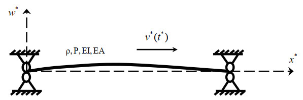
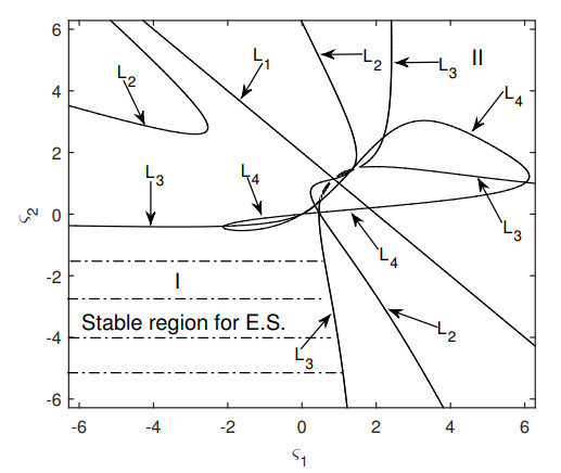
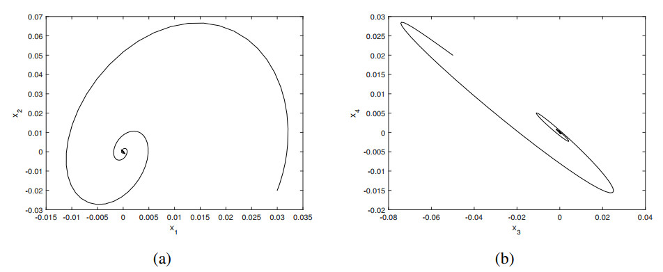
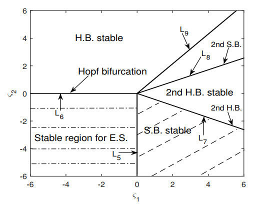
Stability and bifurcation behaviors of an axially moving beam subjected to two frequency excitations were investigated both analytically and numerically. Simultaneous principal parametric resonance as well as combination parametric resonance with 3:1 internal resonance was considered. The critical points are classified into the following categories: a double zero accompanied by two negative eigenvalues, a simple zero coexisting with a pair of pure imaginary eigenvalues, and two pairs of pure imaginary eigenvalues in the non-resonant case. Based on the normal form theory, the stability regions of the initial equilibrium point were studied and the explicit expressions of the critical bifurcation curves for the occurrence of static bifurcation and Hopf bifurcation were obtained. The critical line from which a two-dimensional torus can arise was also discussed. Moreover, numerical simulations were given, which exhibit strong concordance with the analytical predictions. The analytical results obtained here contribute to a better comprehension of the dynamical behaviors of the system and may be helpful to researchers attempting to design the system parameters of related engineering structures.
Citation: Fengxian An, Liangqiang Zhou. Local bifurcation analysis of an accelerating beam subjected to two frequency parametric excitations[J]. AIMS Mathematics, 2025, 10(6): 13409-13431. doi: 10.3934/math.2025602
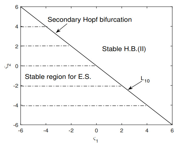
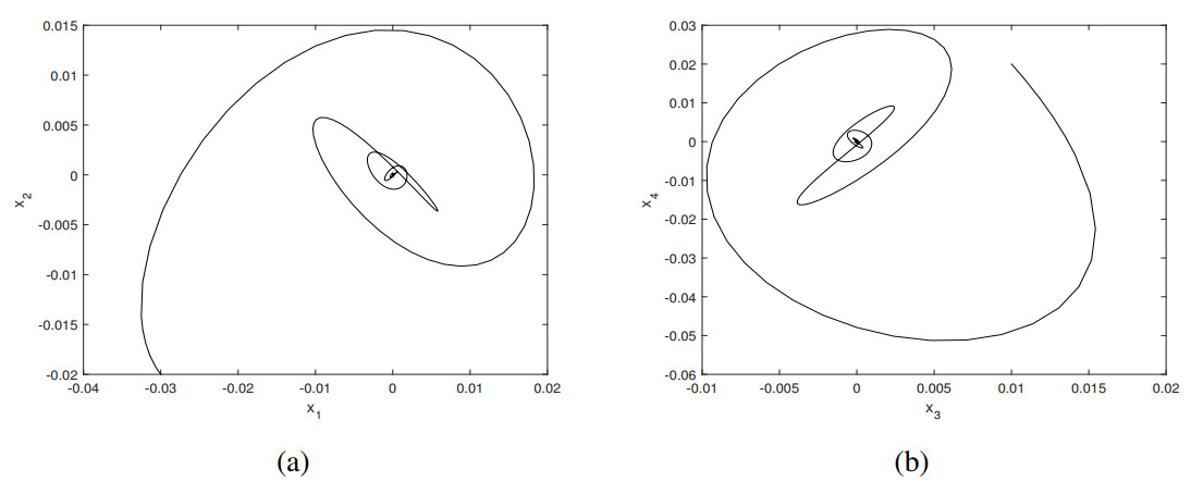
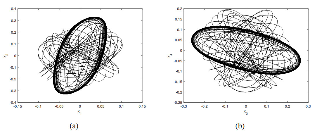
Stability and bifurcation behaviors of an axially moving beam subjected to two frequency excitations were investigated both analytically and numerically. Simultaneous principal parametric resonance as well as combination parametric resonance with 3:1 internal resonance was considered. The critical points are classified into the following categories: a double zero accompanied by two negative eigenvalues, a simple zero coexisting with a pair of pure imaginary eigenvalues, and two pairs of pure imaginary eigenvalues in the non-resonant case. Based on the normal form theory, the stability regions of the initial equilibrium point were studied and the explicit expressions of the critical bifurcation curves for the occurrence of static bifurcation and Hopf bifurcation were obtained. The critical line from which a two-dimensional torus can arise was also discussed. Moreover, numerical simulations were given, which exhibit strong concordance with the analytical predictions. The analytical results obtained here contribute to a better comprehension of the dynamical behaviors of the system and may be helpful to researchers attempting to design the system parameters of related engineering structures.

| [1] |
P. Lad, V. Kartik, Bifurcations and chaos in the dynamics of an axially moving string impacting a distributed unilateral foundation, J. Sound Vib., 589 (2024), 118545. http://dx.doi.org/10.1016/j.jsv.2024.118545 doi: 10.1016/j.jsv.2024.118545

|
| [2] |
Y. D. Hu, Y. X. Tian, Primary parametric resonance, stability analysis and bifurcation characteristics of an axially moving ferromagnetic rectangular thin plate under the action of air-gap field, Nonlinear Dyn., 112 (2024), 8889–8920. http://dx.doi.org/10.1007/s11071-024-09457-3 doi: 10.1007/s11071-024-09457-3
|
| [3] |
L. Chen, Y. Q. Tang, Bifurcation and chaos of axially moving beams under time-varying tension, Chin. J. Theor. Appl. Mech., 51 (2019), 1180–1188. http://dx.doi.org/10.6052/0459-1879-19-068 doi: 10.6052/0459-1879-19-068
|
| [4] |
H. R. Öz, M. Pakdemirli, Two-to-one internal resonances in a shallow curved beam resting on an elastic foundation, Acta Mech., 185 (2006), 245–260. http://dx.doi.org/10.1007/s00707-006-0352-5 doi: 10.1007/s00707-006-0352-5
|
| [5] |
O. O. Ozgumus, M. O. Kaya, Flapwise bending vibration analysis of double tapered rotating Euler-Bernoulli beam by using the differential transform method, Meccanica, 41 (2006), 661–670. http://dx.doi.org/10.1007/s11012-006-9012-z doi: 10.1007/s11012-006-9012-z
|
| [6] |
O. O. Ozgumus, M. O. Kaya, Vibration analysis of a rotating tapered Timoshenko beam using DTM, Meccanica, 45 (2010), 33–42. http://dx.doi.org/10.1007/s11012-009-9221-3 doi: 10.1007/s11012-009-9221-3
|
| [7] |
T. A. Apalara1, A. O. Ige, C. D. Enyi, M. E. Omaba, Uniform stability result of laminated beams with thermoelasticity of type Ⅲ, AIMS Math., 8 (2022), 1090–1101. http://dx.doi.org/10.3934/math.2023054 doi: 10.3934/math.2023054
|
| [8] |
K. Y. Sze, S. H. Chen, J. L. Huang, The incremental harmonic balance method for non-linear vibration of axially moving beams, J. Sound Vib., 281 (2005), 611–626. http://dx.doi.org/10.1016/j.jsv.2004.01.012 doi: 10.1016/j.jsv.2004.01.012
|
| [9] |
X. D. Yang, L. Q. Chen, Bifurcation and chaos of an axially accelerating viscoelastic beam, Chaos Solitons Fract., 23 (2005), 249–258. http://dx.doi.org/10.1016/j.chaos.2004.04.008 doi: 10.1016/j.chaos.2004.04.008
|
| [10] |
C. An, J. Su, Dynamic response of clamped axially moving beams: Integral transform solution, Appl. Math. Comput., 218 (2011), 249–259. http://dx.doi.org/10.1016/j.amc.2011.05.035 doi: 10.1016/j.amc.2011.05.035
|
| [11] |
S. Rajasekaran, Buckling and vibration of axially functionally graded nonuniform beams using differential transformation based dynamic stiffness approach, Meccanica, 48 (2013), 1053–1070. http://dx.doi.org/10.1007/s11012-012-9651-1 doi: 10.1007/s11012-012-9651-1
|
| [12] |
W. Zhang, D. M. Wang, M. H. Yao, Using Fourier differential quadrature method to analyze transverse nonlinear vibrations of an axially accelerating viscoelastic beam, Nonlinear Dyn., 78 (2014), 839–856. http://dx.doi.org/10.1007/s11071-014-1481-3 doi: 10.1007/s11071-014-1481-3
|
| [13] |
Q. Y. Yan, H. Ding, L. Q. Chen, Periodic responses and chaotic behaviors of an axially accelerating viscoelastic Timoshenko beam, Nonlinear Dyn., 78 (2014), 1577–1591. http://dx.doi.org/10.1007/s11071-014-1535-6 doi: 10.1007/s11071-014-1535-6
|
| [14] |
Y. Q. Tang, D. B. Zhang, J. M. Gao, Parametric and internal resonance of axially accelerating viscoelastic beams with the recognition of longitudinally varying tensions, Nonlinear Dyn., 83 (2016), 401–418. http://dx.doi.org/10.1007/s11071-015-2336-2 doi: 10.1007/s11071-015-2336-2
|
| [15] |
A. Moslemi, S. E. Khadem, M. Khazaee, A. Davarpanah, Nonlinear vibration and dynamic stability analysis of an axially moving beam with a nonlinear energy sink, Nonlinear Dyn., 104 (2021), 1955–1972. http://dx.doi.org/10.1007/s11071-021-06389-0 doi: 10.1007/s11071-021-06389-0
|
| [16] |
Y. Hao, H. L. Dai, N. Qiao, L. Wang, Dynamics and stability analysis of an axially moving beam in axial flow, J. Mech. Mater. Struct., 15 (2020), 37–60. http://dx.doi.org/10.2140/jomms.2020.15.37 doi: 10.2140/jomms.2020.15.37
|
| [17] |
L. Chen, Y. Q. Tang, S. Liu, Y. Zhou, X. G. Liu, Nonlinear phenomena in axially moving beams with speed-dependent tension and tension-dependent speed, Int. J. Bifurcat. Chaos, 31 (2021), 2150037. http://dx.doi.org/10.1142/S0218127421500371 doi: 10.1142/S0218127421500371
|
| [18] |
Q. L. Wu, G. Y. Qi, Homoclinic bifurcations and chaotic dynamics of non-planar waves in axially moving beam subjected to thermal load, Appl. Math. Model., 83 (2020), 674–682. http://dx.doi.org/10.1016/j.apm.2020.03.013 doi: 10.1016/j.apm.2020.03.013
|
| [19] |
B. Sahoo, L. N. Panda, G. Pohit, Combination, principal parametric and internal resonances of an accelerating beam under two frequency parametric excitation, Int. J. Non-Linear Mech., 78 (2016), 35–44. http://dx.doi.org/10.1016/j.ijnonlinmec.2015.09.017 doi: 10.1016/j.ijnonlinmec.2015.09.017
|
| [20] |
P. Yu, Analysis on double Hopf bifurcation using computer algebra with the aid of multiple scales, Nonlinear Dyn., 27 (2002), 19–53. http://dx.doi.org/10.1023/A:1017993026651 doi: 10.1023/A:1017993026651
|
Figures(11)

Fengxian An, Liangqiang Zhou. Local bifurcation analysis of an accelerating beam subjected to two frequency parametric excitations[J]. AIMS Mathematics, 2025, 10(6): 13409-13431. doi: 10.3934/math.2025602


 DownLoad: