Minimum span frequency allocation problem: A vector bin packing approach

Ki-Hun Lee; Hyang-Won Lee; Bang Chul Jung; Ki-Hun Lee; Hyang-Won Lee; Bang Chul Jung

doi:10.3934/math.2025595

AIMS Mathematics

2025, Volume 10, Issue 6: 13278-13295. doi: 10.3934/math.2025595

Previous Article Next Article

Research article Special Issues

Minimum span frequency allocation problem: A vector bin packing approach

1.
Department of AI Convergence, Kunsan National University, Gunsan 54150, South Korea
2.
Department of Computer Science and Engineering, Konkuk University, Seoul 05029, South Korea
3.
Department of Electrical and Computer Engineering, Ajou University, Suwon 16499, South Korea

Received: 20 January 2025 Revised: 14 May 2025 Accepted: 29 May 2025 Published: 10 June 2025
MSC : 90C05, 90C27

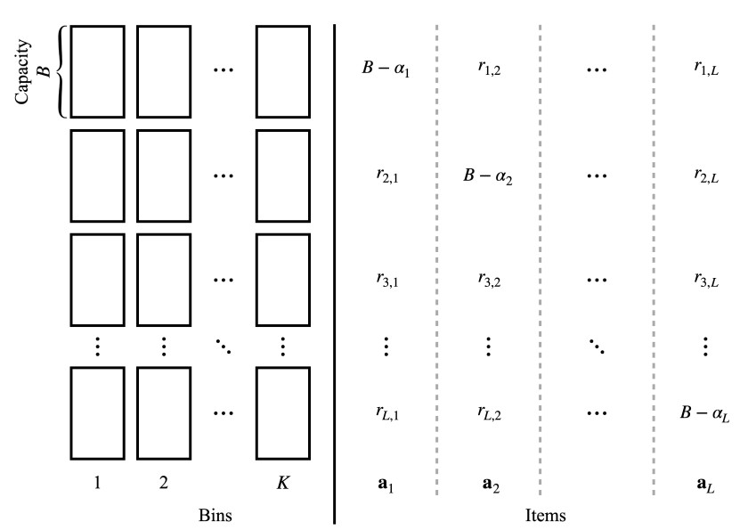
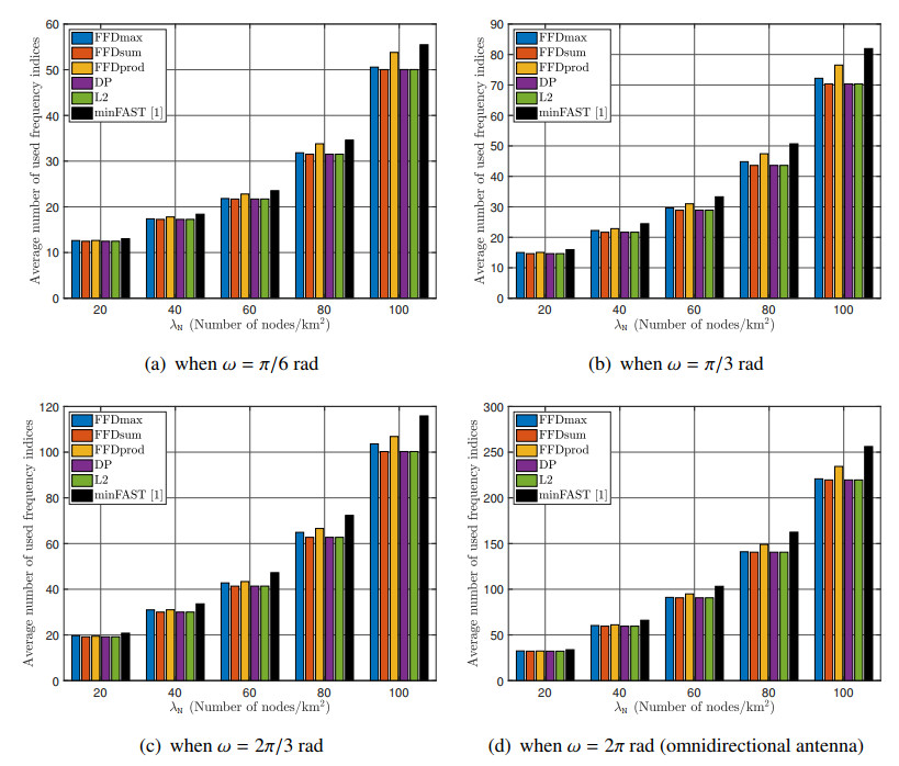
We revisit the minimum span frequency allocation problem (MS-FAP) to address the spectrum scarcity issue in wireless communication networks. The MS-FAP seeks to minimize the gap (span) between the highest and lowest frequencies used, thereby reducing the total bandwidth required in the network while ensuring the demand of each associated link. We formulate the MS-FAP with the physical interference model as a vector bin packing (VBP) problem on a weighted complete directed graph and then leverage conventional heuristic algorithms based on first-fit decreasing (FFD). Extensive computer simulations and analysis results demonstrate that the FFD-based heuristics outperform the state-of-the-art MS-FA algorithm in both performance and computational complexity. In particular, the FFDsum, an item-centric FFD algorithm, generally achieves the best performance for the MS-FAP. This work is noteworthy in that it is the first to apply VBP to the MS-FAP.
- first-fit-decreasing,
- heuristics,
- minimum span frequency allocation,
- radio resource management,
- vector bin packing,
- wireless network
Citation: Ki-Hun Lee, Hyang-Won Lee, Bang Chul Jung. Minimum span frequency allocation problem: A vector bin packing approach[J]. AIMS Mathematics, 2025, 10(6): 13278-13295. doi: 10.3934/math.2025595

Related Papers:

Abstract

We revisit the minimum span frequency allocation problem (MS-FAP) to address the spectrum scarcity issue in wireless communication networks. The MS-FAP seeks to minimize the gap (span) between the highest and lowest frequencies used, thereby reducing the total bandwidth required in the network while ensuring the demand of each associated link. We formulate the MS-FAP with the physical interference model as a vector bin packing (VBP) problem on a weighted complete directed graph and then leverage conventional heuristic algorithms based on first-fit decreasing (FFD). Extensive computer simulations and analysis results demonstrate that the FFD-based heuristics outperform the state-of-the-art MS-FA algorithm in both performance and computational complexity. In particular, the FFDsum, an item-centric FFD algorithm, generally achieves the best performance for the MS-FAP. This work is noteworthy in that it is the first to apply VBP to the MS-FAP.

References

[1]	K. H. Lee, H. W. Lee, H. Lee, S. H. Chae, Y. Kim, B. C. Jung, minFAST: Minimum span frequency assignment technique for integrated access and backhaul networks, IEEE Trans. Veh. Technol., 72 (2023), 8222–8227. https://doi.org/10.1109/TVT.2023.3243886 doi: 10.1109/TVT.2023.3243886
[2]	M. Mohammadi, Z. Mobini, D. Galappaththige, C. Tellambura, A comprehensive survey on full-duplex communication: Current solutions, future trends, and open issues, IEEE Commun. Surveys Tuts., 25 (2023), 2190–2244. https://doi.org/10.1109/COMST.2023.3318198 doi: 10.1109/COMST.2023.3318198
[3]	S. Biswas, A. Bishnu, F. A. Khan, T. Ratnarajah, In-band full-duplex dynamic spectrum sharing in beyond 5G networks, IEEE Commun. Mag., 59 (2021), 54–60. https://doi.org/10.1109/MCOM.001.2000929 doi: 10.1109/MCOM.001.2000929
[4]	Y. Kim, H. J. Moon, H. Yoo, B. Kim, K. K. Wong, C. B. Chae, A state-of-the-art survey on full-duplex network design, Proc. IEEE, 112 (2024), 463–486. https://doi.org/10.1109/JPROC.2024.3363218 doi: 10.1109/JPROC.2024.3363218
[5]	M. Song, C. Xin, Y. Zhao, X. Cheng, Dynamic spectrum access: From cognitive radio to network radio, IEEE Wirel. Commun., 19 (2012), 23–29. https://doi.org/10.1109/MWC.2012.6155873 doi: 10.1109/MWC.2012.6155873
[6]	T. S. Rappaport, Y. Xing, O. Kanhere, S. Ju, A. Madanayake, S Mandal, et al., Wireless communications and applications above 100 GHz: Opportunities and challenges for 6G and beyond, IEEE Access, 7 (2019), 78729–78757. https://doi.org/10.1109/ACCESS.2019.2921522 doi: 10.1109/ACCESS.2019.2921522
[7]	C. I. Páez-Rueda, A. Fajardo, M. Pérez, G. Yamhure, G. Perilla, The F/DR-D-10 algorithm: A novel heuristic strategy to solve the minimum span frequency assignment problem embedded in mobile applications, Mathematics, 11 (2023), 4243. https://doi.org/10.3390/math11204243 doi: 10.3390/math11204243
[8]	K. H. Lee, S. Lee, J. Park, H. Lee, B. C. Jung, MUSCAT: Distributed multi-agent $Q$-learning-based minimum span channel allocation technique for UAV-enabled wireless networks, Comput. Netw., 247 (2024), 100462. https://doi.org/10.1016/j.comnet.2024.110462 doi: 10.1016/j.comnet.2024.110462
[9]	K. I. Aardal, S. P. M. van Hoesel, A. M. C. A. Koster, C. Mannino, A. Sassano, Models and solution techniques for frequency assignment problems, Ann. Oper. Res., 153 (2007), 79–129. https://doi.org/10.1007/s10479-007-0178-0 doi: 10.1007/s10479-007-0178-0
[10]	A. N. Rouskas, M. G. Kazantzakis, M. E. Anagnostou, Minimization of frequency assignment span in cellular networks, IEEE Trans. Veh. Technol., 48 (1999), 873–882. https://doi.org/doi/10.1109/25.765004 doi: 10.1109/25.765004
[11]	A. Avenali, C. Mannino, A. Sassano, Minimizing the span of $d$-walks to compute optimum frequency assignments, Math. Program., 91 (2002), 357–374. https://doi.org/10.1007/s101070100247 doi: 10.1007/s101070100247
[12]	S. M. Allen, D. H. Smith, S. Hurley, Generation of lower bounds for minimum span frequency assignment, Discrete Appl. Math., 119 (2002), 59–78. https://doi.org/10.1016/S0166-218X(01)00265-7 doi: 10.1016/S0166-218X(01)00265-7
[13]	R. Montemanni, D. H. Smith, S. M. Allen, An ANTS algorithm for the minimum-span frequency-assignment problem with multiple interference, IEEE Trans. Veh. Technol., 51 (2002), 949–953. https://doi.org/10.1109/TVT.2002.800634 doi: 10.1109/TVT.2002.800634
[14]	B. Dias, R. Freitas, N. Maculan, P. Michelon, Integer and constraint programming approaches for providing optimality to the bandwidth multicoloring problem, RAIRO-Oper. Res., 55 (2021), S1949–S1967. https://doi.org/10.1051/ro/2020065 doi: 10.1051/ro/2020065
[15]	K. H. Lee, Y. J. Song, J. H. Hwang, B. C. Jung, Minimum span frequency allocation technique for 6G in-band full-duplex IAB networks, In: 2024 15th International Conference on Information and Communication Technology Convergence (ICTC), 2024. https://doi.org/10.1109/ICTC62082.2024.10827345
[16]	R. Panigrahy, K. Talwar, L. Uyeda, U. Wieder, Heuristics for vector bin packing, technical Report, Microsoft Research, 2011. Available from: https://www.microsoft.com/en-us/research/publication/heuristics-for-vector-bin-packing/.
[17]	L. Nagel, N. Popov, T. Süß, Z. Wang, Analysis of heuristics for vector scheduling and vector bin packing, In: M. Sellmann, K. Tierney (eds), Learning and Intelligent Optimization-17th International Conference (LION 17), Springer, Cham, 2023. https://doi.org/10.1007/978-3-031-44505-7_39
[18]	H. I. Christensen, A. Khan, S. Pokutta, P. Tetali, Approximation and online algorithms for multidimensional bin packing: A survey, Comput. Sci. Rev., 24 (2017), 63–79. https://doi.org/10.1016/j.cosrev.2016.12.001 doi: 10.1016/j.cosrev.2016.12.001
[19]	A. Kulik, M. Mnich, H. Shachnai, Improved approximations for vector bin packing via iterative randomized rounding, In: 2023 IEEE 64th Annual Symposium on Foundations of Computer Science (FOCS), 2023. https://doi.org/10.1109/FOCS57990.2023.00084
[20]	H. I. Christensen, A. Khan, S. Pokutta, P. Tetali, Multidimensional bin packing and other related problems: A survey, 2016. Available from: https://api.semanticscholar.org/CorpusID: 9048170.
[21]	D. S. Johnson, Vector bin packing, In: Encyclopedia of Algorithms, New York: Springer, 2016. https://doi.org/10.1007/978-1-4939-2864-4_495
[22]	K. H. Lee, H. W. Lee, H. Lee, B. C. Jung, PRADA: Practical access point deployment algorithm for cell-free industrial IoT networks, In: 2023 IEEE 20th Consumer Communications & Networking Conference (CCNC), 2023. https://doi.org/10.1109/CCNC51644.2023.10060457
[23]	J. Ben-Othman, L. Mokdad, M. O. Cheikh, A new architecture of wireless mesh networks based IEEE 802.11s directional antennas, In: 2011 IEEE International Conference on Communications (ICC), 2011. https://doi.org/10.1109/icc.2011.5962994
[24]	J. Wildman, P. H. J. Nardelli, M. Latva-aho, S. Weber, On the joint impact of beamwidth and orientation error on throughput in directional wireless Poisson networks, IEEE Trans. Wirel. Commun., 13 (2014), 7072–7085. https://doi.org/10.1109/TWC.2014.2331055 doi: 10.1109/TWC.2014.2331055
[25]	G. Naik, J. M. Park, J. Ashdown, W. Lehr, Next generation Wi-Fi and 5G NR-U in the 6 GHz bands: Opportunities and challenges, IEEE Access, 8 (2020), 153027–153056. https://doi.org/10.1109/ACCESS.2020.3016036 doi: 10.1109/ACCESS.2020.3016036

Reader Comments

Your name:*

Email:*
© 2025 the Author(s), licensee AIMS Press. This is an open access article distributed under the terms of the Creative Commons Attribution License (http://creativecommons.org/licenses/by/4.0)