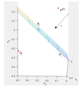
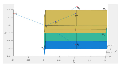
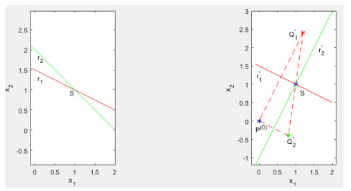
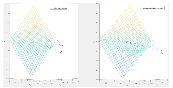
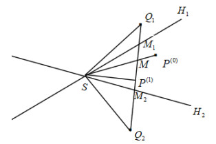
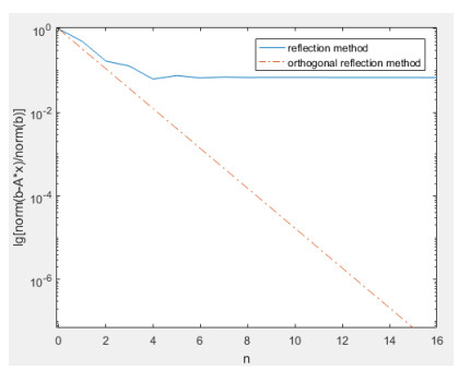
This paper extends the convergence analysis of the reflection method from the case of $ 2 $ equations to the case of $ n $ equations. A novel approach called the orthogonal reflection method is also proposed. The orthogonal reflection method comprises two key steps. First, a Householder transformation is employed to derive an equivalent system of equations with an orthogonal coefficient matrix that maintains the same solution set as the original system. Second, the reflection method is applied to efficiently solve this transformed system. Compared with the reflection method, the orthogonal reflection method significantly enhances the convergence speed, especially when the angles are acute between the hyperplanes represented by the linear system. We also derive the convergence rate for it, demonstrating that the orthogonal reflection method is always convergent for an arbitrary point in $ \mathbb{R}^n $. The necessity of orthogonalization is presented in the form of a theorem in $ \mathbb{R}^2 $. When the coefficient matrix has a large condition number, the orthogonal reflection method can still compute relatively accurate numerical solutions rapidly. By comparing with algorithms including Jacobi iteration, Gauss-Seidel iteration, the conjugate gradient method, GMRES, weighted RBAS, and the reflection method on coefficient matrices of 10×10 random matrices, 1000×1000 sparse matrices, and 1000×1000 randomly generated full-rank matrices, the efficiency and robustness of the orthogonal reflection method are demonstrated.
Citation: Wenyue Feng, Hailong Zhu. The orthogonal reflection method for the numerical solution of linear systems[J]. AIMS Mathematics, 2025, 10(6): 12888-12899. doi: 10.3934/math.2025579
This paper extends the convergence analysis of the reflection method from the case of $ 2 $ equations to the case of $ n $ equations. A novel approach called the orthogonal reflection method is also proposed. The orthogonal reflection method comprises two key steps. First, a Householder transformation is employed to derive an equivalent system of equations with an orthogonal coefficient matrix that maintains the same solution set as the original system. Second, the reflection method is applied to efficiently solve this transformed system. Compared with the reflection method, the orthogonal reflection method significantly enhances the convergence speed, especially when the angles are acute between the hyperplanes represented by the linear system. We also derive the convergence rate for it, demonstrating that the orthogonal reflection method is always convergent for an arbitrary point in $ \mathbb{R}^n $. The necessity of orthogonalization is presented in the form of a theorem in $ \mathbb{R}^2 $. When the coefficient matrix has a large condition number, the orthogonal reflection method can still compute relatively accurate numerical solutions rapidly. By comparing with algorithms including Jacobi iteration, Gauss-Seidel iteration, the conjugate gradient method, GMRES, weighted RBAS, and the reflection method on coefficient matrices of 10×10 random matrices, 1000×1000 sparse matrices, and 1000×1000 randomly generated full-rank matrices, the efficiency and robustness of the orthogonal reflection method are demonstrated.

| [1] |
A. M. Childs, R. Kothari, R. D. Somma, Quantum algorithm for systems of linear equations with exponentially improved dependence on precision, SIAM J. Comput., 46 (2017), 1920–1950. https://doi.org/10.1137/16M1087072 doi: 10.1137/16M1087072

|
| [2] |
E. Carson, N. J. Higham, Accelerating the solution of linear systems by iterative refinement in three precisions, SIAM J. Sci. Comput., 40 (2018), 817–847. https://doi.org/10.1137/17m1140819 doi: 10.1137/17m1140819
|
| [3] |
N. J. Higham, S. Pranesh, Exploiting lower precision arithmetic in solving symmetric positive definite linear systems and least squares problem, SIAM J. Sci. Comput., 43 (2021), 258–277. https://doi.org/10.1137/19M1298263 doi: 10.1137/19M1298263
|
| [4] |
T. A. Davis, S. Rajamanickam, W. M. S. Lakhdar, A survey of direct methods for sparse linear systems, Acta Numer., 25 (2016), 383–566. https://doi.org/10.1017/S0962492916000076 doi: 10.1017/S0962492916000076
|
| [5] | H. A. V. D. Vorst, Computer solution of large linear systems, Elsevier, 1999. https://doi.org/10.1016/0377-0427(94)90302-6 |
| [6] |
Z. Zlatev, Use of iterative refinement in the solution of sparse linear systems, SIAM J. Numer. Anal., 19 (1982), 381–399. https://doi.org/10.1137/0719024 doi: 10.1137/0719024
|
| [7] |
H. Y. Huang, A direct method for the general solution of a system of linear equations, J. Optimiz. Theory Appl., 16 (1975), 429–445. https://doi.org/10.1007/bf00933852 doi: 10.1007/bf00933852
|
| [8] |
E. Spedicato, M. T. Vespucci, Variations on the Gram-Schmidt and the Huang algorithms for linear systems: A numerical study, Appl. Math., 38 (1993), 81–100. https://doi.org/10.21136/AM.1993.104537 doi: 10.21136/AM.1993.104537
|
| [9] | D. M. Young, Iterative solution of large linear systems, Elsevier, 2014. |
| [10] |
V. Simoncini, D. B. Szyld, Recent developments in Krylov subspace methods for linear systems, Numer. Linear Algebr., 14 (2007), 1–59. https://doi.org/10.1002/nla.499 doi: 10.1002/nla.499
|
| [11] |
L. Tondji, D. A. Lorenz, Faster randomized block sparse Kaczmarz by averaging, Numer. Algorithms, 93 (2023), 1417–1451. https://doi.org/10.1007/s11075-022-01473-x doi: 10.1007/s11075-022-01473-x
|
| [12] |
V. Patel, M. Jahangoshahi, D. A. Maldonado, Randomized block adaptive linear system solvers, SIAM J. Matrix Anal. A., 44 (2023), 1349–1369. https://doi.org/10.1137/22M1488715 doi: 10.1137/22M1488715
|
| [13] |
M. Guida, C. Sbordone, The reflection method for the numerical solution of linear systems, SIAM Rev., 65 (2023), 1137–1151. https://doi.org/10.1137/22M1470463 doi: 10.1137/22M1470463
|
| [14] | G. Cimmino, Approximate computation of the solutions of systems of linear equations, Rend. Accad. Sci. Fis. Mat. Napoli, 89 (2022), 65–72. |
| [15] | M. Benzi, Gianfranco Cimmino's contributions to numerical mathematics, Atti del Seminario di Analisi Matematica, Dipartimento di Matematica dell'Universita di Bologna. Volume Speciale: Ciclo di Conferenze in Ricordo di Gianfranco Cimmino, 2004, 87–109. |
| [16] |
Y. Censor, T. Elfving, New methods for linear inequalities, Linear Algebra Appl., 42 (1982), 199–211. https://doi.org/10.1016/0024-3795(82)90149-5 doi: 10.1016/0024-3795(82)90149-5
|
| [17] |
T. Elfving, A projection method for semidefinite linear systems and its applications, Linear Algebra Appl., 391 (2004), 57–73. https://doi.org/10.1016/j.laa.2003.11.025 doi: 10.1016/j.laa.2003.11.025
|
| [18] |
Y. Censor, M. D. Altschuler, W. D. Powlis, On the use of Cimmino's simultaneous projections method for computing a solution of the inverse problem in radiation therapy treatment planning, Inverse Probl., 4 (1988), 607. https://doi.org/10.1088/0266-5611/4/3/006 doi: 10.1088/0266-5611/4/3/006
|
| [19] | S. Petra, C. Popa, C. Schn$\ddot{o}$rr, Extended and constrained Cimmino-type algorithms with applications in tomographic image reconstruction, Universitatsbibliothek Heidelberg, 2008. https://doi.org/10.11588/heidok.00008798 |
| [20] |
M. R. Hestenes, E. Stiefel, Methods of conjugate Gradients for solving linear systems, J. Res. Natl. Bureau Stand., 49 (1952), 409–436. https://doi.org/10.6028/jres.049.044 doi: 10.6028/jres.049.044
|
Figures(6) / Tables(3)

Wenyue Feng, Hailong Zhu. The orthogonal reflection method for the numerical solution of linear systems[J]. AIMS Mathematics, 2025, 10(6): 12888-12899. doi: 10.3934/math.2025579


 DownLoad: