Soliton solutions of the nonlinear dynamics in the Boussinesq equation with bifurcation analysis and chaos

Muhammad Shakeel; Amna Mumtaz; Abdul Manan; Marouan Kouki; Nehad Ali Shah; Muhammad Shakeel; Amna Mumtaz; Abdul Manan; Marouan Kouki; Nehad Ali Shah

doi:10.3934/math.2025484

AIMS Mathematics

2025, Volume 10, Issue 5: 10626-10649. doi: 10.3934/math.2025484

Previous Article Next Article

Research article Special Issues

Soliton solutions of the nonlinear dynamics in the Boussinesq equation with bifurcation analysis and chaos

1.
Department of Mathematics, Faculty of Basic Sciences, University of Wah, Wah Cantt 47040, Pakistan; muhammad.shakeel@uow.edu.pk; amna.mumtazsyed@gmail.com
2.
Department of Mathematics, Faculty of Sciences, Superior University, Main Campus Lahore, Pakistan; abdul.manan@superior.edu.pk
3.
Department of Information System, Faculty of Computing and Information Technology, Northern Border University, Rafha, Saudi Arabia
4.
Department of Mechanical Engineering, Sejong University, Seoul 05006, Republic of Korea
^a These authors contributed equally to this work and are co-first authors

Received: 13 February 2025 Revised: 08 April 2025 Accepted: 18 April 2025 Published: 09 May 2025
MSC : 39A33, 35A20, 34G20

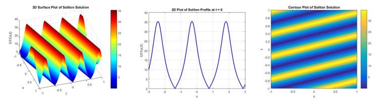
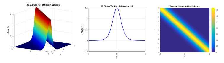
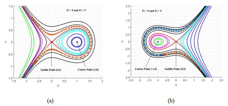
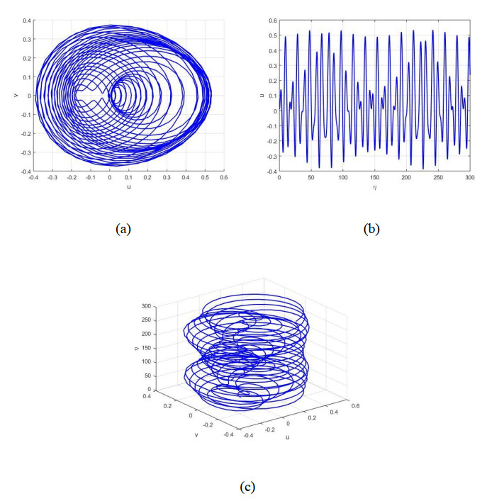
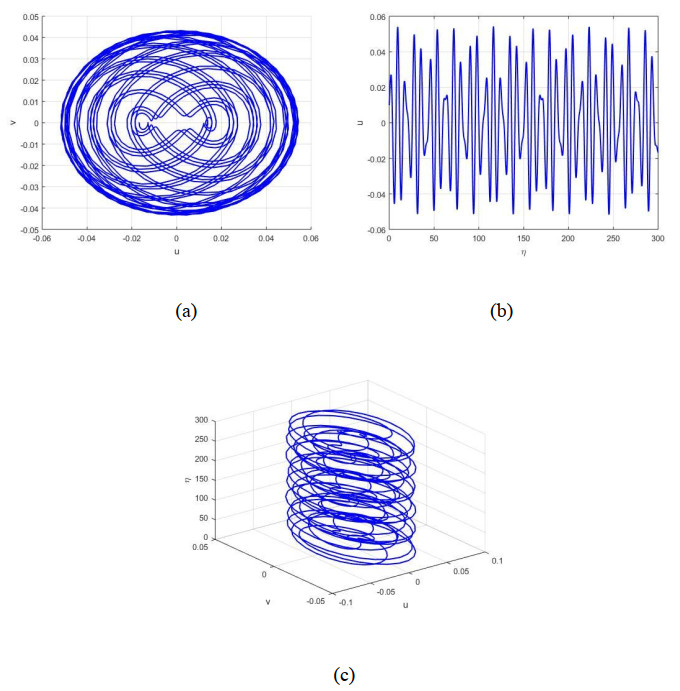
In this study, we examined the nonlinear dynamics of the Boussinesq equation, a foundational equation in ocean engineering to model and investigate the behavior of waves in shallow water. The novel (G'/G²)-expansion method was employed to obtain different soliton solutions, including periodic, bright, W-type, and bell-shaped soliton solutions. These solutions are illustrated through 2D, 3D, and contour plots. We discovered different dynamical behavior, including periodic, quasi-periodic, and weak chaos, depending on the choice of initial conditions and parameters. The important outcomes included the detection of multistable attractors and the presence of weak chaotic behavior supported by Lyapunov exponents. These understandings have important effects in practical uses such as energy harvesting and wave control in ocean systems, where handling and understanding system transitions and stability is crucial. These findings also give a framework for further examination of stability and control in nonlinear wave systems.
- Boussinesq equation,
- novel (G'/G²)-expansion method,
- phase portrait,
- chaotic analysis,
- Lyapunov exponents
Citation: Muhammad Shakeel, Amna Mumtaz, Abdul Manan, Marouan Kouki, Nehad Ali Shah. Soliton solutions of the nonlinear dynamics in the Boussinesq equation with bifurcation analysis and chaos[J]. AIMS Mathematics, 2025, 10(5): 10626-10649. doi: 10.3934/math.2025484

Related Papers:

Abstract

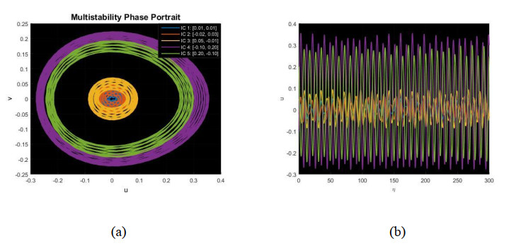
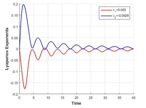
In this study, we examined the nonlinear dynamics of the Boussinesq equation, a foundational equation in ocean engineering to model and investigate the behavior of waves in shallow water. The novel (G'/G²)-expansion method was employed to obtain different soliton solutions, including periodic, bright, W-type, and bell-shaped soliton solutions. These solutions are illustrated through 2D, 3D, and contour plots. We discovered different dynamical behavior, including periodic, quasi-periodic, and weak chaos, depending on the choice of initial conditions and parameters. The important outcomes included the detection of multistable attractors and the presence of weak chaotic behavior supported by Lyapunov exponents. These understandings have important effects in practical uses such as energy harvesting and wave control in ocean systems, where handling and understanding system transitions and stability is crucial. These findings also give a framework for further examination of stability and control in nonlinear wave systems.

References

[1]	A. J. Grass, Sediments transport by waves and currents, University College, London, Department of Civil Engineering, 1981.
[2]	S. Qian, G. Li, F. Shao, Q. Niu, Well-balanced central WENO schemes for the sediment transport model in shallow water, Comput. Geosci., 22 (2018), 763–773. https://doi.org/10.1007/s10596-018-9724-x doi: 10.1007/s10596-018-9724-x
[3]	M. J. Castro Diáz, E. D. Fernández-Nieto, A. M. Ferreiro, Sediment transport models in shallow water equations and numerical approach by high order finite volume methods, Comput. Fluids, 37 (2008), 299–316. https://doi.org/10.1016/j.compfluid.2007.07.017 doi: 10.1016/j.compfluid.2007.07.017
[4]	M. De Vries, Considerations about non-steady bed-load-transport in open channels, Tech. Rep., Hydraulics Laboratory, Delft, the Netherlands, 1965.
[5]	A. Armanini, Principles of river hydraulics, Springer, 1 Ed., Springer International Publishing, 2018. https://doi.org/10.1007/978-3-319-68101-6
[6]	S. Mayer, A. Garapon, L. S. Sørensen, A fractional step method for unsteady free-surface flow with applications to non-linear wave dynamics, Int. J. Numer. Methods Fluids, 28 (1998), 293–315. https://doi.org/10.1002/(SICI)1097-0363(19980815)28:2 < 293::AID-FLD719 > 3.0.CO; 2-1 doi: 10.1002/(SICI)1097-0363(19980815)28:2 < 293::AID-FLD719 > 3.0.CO; 2-1
[7]	K. J. Wang, F. Shi, S. Li, P. Xu, Dynamics of resonant soliton, novel hybrid interaction, complex N-soliton and the abundant wave solutions to the (2+1)-dimensional Boussinesq equation, Alex. Eng. J., 105 (2024), 485–495. https://doi.org/10.1016/j.aej.2024.08.015 doi: 10.1016/j.aej.2024.08.015
[8]	L. Xu, X. Yin, N. Cao, S. Bai, Multi-soliton solutions of a variable coefficient Schrödinger equation derived from vorticity equation, Nonlinear Dyn., 112 (2024), 2197–2208. https://doi.org/10.1007/s11071-023-09158-3 doi: 10.1007/s11071-023-09158-3
[9]	A. Ali, A. R. Seadawy, Dispersive soliton solutions for shallow water wave system and modified Benjamin-Bona-Mahony equations via applications of mathematical methods, J. Ocean Eng. Sci., 6 (2021), 85–98. https://doi.org/10.1016/j.joes.2020.06.001 doi: 10.1016/j.joes.2020.06.001
[10]	M. Safari, D. D. Ganji, M. Moslemi, Application of He's variational iteration method and Adomian's decomposition method to the fractional KdV-Burgers-Kuramoto equation, Comput. Math. Appl., 58 (2009), 2091–2097. https://doi.org/10.1016/j.camwa.2009.03.043 doi: 10.1016/j.camwa.2009.03.043
[11]	H. O. Roshid, M. A. Akbar, M. N. Alam, M. F. Hoque, N. Rahman, New extended (G'/G)-expansion method to solve nonlinear evolution equation: the (3 + 1)-dimensional potential-YTSF equation, SpringerPlus, 3 (2014), 122. https://doi.org/10.1186/2193-1801-3-122 doi: 10.1186/2193-1801-3-122
[12]	M. M. Miah, H. M. Shahadat Ali, M. Ali Akbar, A. M. Wazwaz, Some applications of the (G'/G, 1/G)-expansion method to find new exact solutions of NLEEs, Eur. Phys. J. Plus, 132 (2017), 252. https://doi.org/10.1140/epjp/i2017-11571-0 doi: 10.1140/epjp/i2017-11571-0
[13]	H. Naher, F. A. Abdullah, The basic (G'/G)-expansion method for the fourth order Boussinesq equation, Appl. Math., 3 (2012), 1144–1152. http://doi.org/10.4236/am.2012.310168
[14]	K. Ayub, M. Saeed, M. Ashraf, M. Yaqub, Q. M. Hassan, Soliton solutions of variant Boussinesq equations through exp-function method, Univ. Wah J. Sci. Technol., 1 (2017), 24–30.
[15]	S. Kaewta, S. Sirisubtawee, S. Koonprasert, S. Sungnul, Applications of the (G'/G²)-expansion method for solving certain nonlinear conformable evolution equations, Fractal Fract., 5 (2021), 88. https://doi.org/10.3390/fractalfract5030088 doi: 10.3390/fractalfract5030088
[16]	C. Jipei, C. Hao, The (g'/g²)-expansion method and its application to coupled nonlinear Klein-Gordon equation, J. South China Normal Univ., 44 (2012), 63–66.
[17]	K. Zhouzheng, (G'/G²)-expansion solutions to MBBM and OBBM equations, J. Partial Differ. Equ., 28 (2015), 158–166. https://doi.org/10.4208/jpde.v28.n2.5 doi: 10.4208/jpde.v28.n2.5
[18]	P. Devi, K. Singh, Exact traveling wave solutions of the (2+1)-dimensional Boiti-Leon-Pempinelli system using (G'/G²)-expansion method, AIP Conf. Proc., 2214 (2020), 020030. https://doi.org/10.1063/5.0003694 doi: 10.1063/5.0003694
[19]	M. Shakeel, N. A. Shah, J. D. Chung, Novel analytical technique to find closed form solutions of time fractional partial differential equations, Fractal Fract., 6 (2022), 24. https://doi.org/10.3390/fractalfract6010024 doi: 10.3390/fractalfract6010024
[20]	S. Behera, N. H. Aljahdaly, J. P. S. Virdi, On the modified (G'/G²)-expansion method for finding some analytical solutions of the traveling waves, J. Ocean Eng. Sci., 7 (2022), 313–320. https://doi.org/10.1016/j.joes.2021.08.013 doi: 10.1016/j.joes.2021.08.013
[21]	N. H. Aljahdaly, Some applications of the modified (G'/G²)-expansion method in mathematical physics, Results Phys., 13 (2019), 102272. https://doi.org/10.1016/j.rinp.2019.102272 doi: 10.1016/j.rinp.2019.102272
[22]	A. Mumtaz, M. Shakeel, M. Alshehri, N. A. Shah, New analytical technique for prototype closed form solutions of certain nonlinear partial differential equations, Results Phys., 60 (2024), 107640. https://doi.org/10.1016/j.rinp.2024.107640 doi: 10.1016/j.rinp.2024.107640
[23]	R. Ali, S. Barak, A. Altalbe, Analytical study of soliton dynamics in the realm of fractional extended shallow water wave equations, Phys. Scr., 99 (2024), 065235. https://doi.org/10.1088/1402-4896/ad4784 doi: 10.1088/1402-4896/ad4784
[24]	M. U. D. Junjua, S. Altaf, A. A. Alderremy, E. E. Mahmoud, Exact wave solutions of truncated M-fractional Boussinesq-Burgers system via an effective method, Phys. Scr., 99 (2024), 095263. https://doi.org/10.1088/1402-4896/ad6ec9 doi: 10.1088/1402-4896/ad6ec9
[25]	T. B. Benjamin, J. L. Bona, J. J. Mahony, Model equations for long waves in nonlinear dispersive systems, Philos. Trans. R. Soc. Lond Ser. A, Math. Phys. Sci., 272 (1972), 47–78. https://doi.org/10.1098/rsta.1972.0032 doi: 10.1098/rsta.1972.0032
[26]	D. H. Peregrine, Calculations of the development of an undular bore, J. Fluid Mech., 25 (1966), 321–330. https://doi.org/10.1017/S0022112066001678 doi: 10.1017/S0022112066001678
[27]	M. T. Darvishi, M. Najafi, A. M. Wazwaz, Soliton solutions for Boussinesq-like equations with spatio-temporal dispersion, Ocean Eng., 130 (2017), 228–240. https://doi.org/10.1016/j.oceaneng.2016.11.052 doi: 10.1016/j.oceaneng.2016.11.052
[28]	S. W. Yao, L. Akinyemi, M. Mirzazadeh, M. Inc, K. Hosseini, M. Şenol, Dynamics of optical solitons in higher-order Sasa–Satsuma equation, Results Phys., 30 (2021), 104825. https://doi.org/10.1016/j.rinp.2021.104825 doi: 10.1016/j.rinp.2021.104825
[29]	A. Jhangeer, H. Almusawa, Z. Hussain, Bifurcation study and pattern formation analysis of a nonlinear dynamical system for chaotic behavior in travelling wave solution, Results Phys., 37 (2022), 105492. https://doi.org/10.1016/j.rinp.2022.105492 doi: 10.1016/j.rinp.2022.105492
[30]	Z. U. Rehman, Z. Hussain, Z. Li, T. Abbas, I. Tlili, Bifurcation analysis and multi-stability of chirped form optical solitons with phase portrait, Results Eng., 21 (2024), 101861. https://doi.org/10.1016/j.rineng.2024.101861 doi: 10.1016/j.rineng.2024.101861
[31]	H. Almusawa, M. Y. Almusawa, A. Jhangeer, Z. Hussain, Exploring nonlinear dynamics in intertidal water waves: Insights from fourth-order Boussinesq equations, Axioms, 13 (2024), 793. https://doi.org/10.3390/axioms13110793 doi: 10.3390/axioms13110793
[32]	S. N. Chow, J. K. Hale, Methods of bifurcation theory, 1 Ed., Springer New York, 1982. https://doi.org/10.1007/978-1-4613-8159-4
[33]	M. B. Riaz, A. Jhangeer, F. Z. Duraihem, J. Martinovic, Analyzing dynamics: Lie symmetry approach to bifurcation, chaos, multistability, and solitons in extended (3+1)-dimensional wave equation, Symmetry, 16 (2024), 608. https://doi.org/10.3390/sym16050608 doi: 10.3390/sym16050608
[34]	K. J. Wang, G. D. Wang, F. Shi, X. L. Liu, H. W. Zhu, Variational principle, Hamiltonian, bifurcation analysis, chaotic behaviours and the diverse solitary wave solutions of the simplified modified Camassa–Holm equation, Int. J. Geom. Methods Mod. Phys., 2025, 2550013. https://doi.org/10.1142/S0219887825500136 doi: 10.1142/S0219887825500136
[35]	A. Jhangeer, Beenish, Study of magnetic fields using dynamical patterns and sensitivity analysis, Chaos Soliton. Fract., 182 (2024), 114827. https://doi.org/10.1016/j.chaos.2024.114827 doi: 10.1016/j.chaos.2024.114827
[36]	A. Jhangeer, W. A. Faridi, M. Alshehri, The study of phase portraits, multistability visualization, Lyapunov exponents and chaos identification of coupled nonlinear volatility and option pricing model, Eur. Phys. J. Plus, 139 (2024), 658. https://doi.org/10.1140/epjp/s13360-024-05435-1 doi: 10.1140/epjp/s13360-024-05435-1
[37]	A. Wolf, J. B. Swift, H. L. Swinney, J. A. Vastano, Determining Lyapunov exponents from a time series, Phys. D, 16 (1985), 285–317. https://doi.org/10.1016/0167-2789(85)90011-9 doi: 10.1016/0167-2789(85)90011-9

Reader Comments

Your name:*

Email:*
© 2025 the Author(s), licensee AIMS Press. This is an open access article distributed under the terms of the Creative Commons Attribution License (http://creativecommons.org/licenses/by/4.0)