Bayesian estimation and prediction for linear exponential models using ordered moving extremes ranked set sampling in medical data

Haidy A. Newer; Bader S Alanazi; Haidy A. Newer; Bader S Alanazi

doi:10.3934/math.2025055

AIMS Mathematics

2025, Volume 10, Issue 1: 1162-1182. doi: 10.3934/math.2025055

Previous Article Next Article

Research article Special Issues

Bayesian estimation and prediction for linear exponential models using ordered moving extremes ranked set sampling in medical data

Haidy A. Newer ^{1
,
,},
Bader S Alanazi ²

1.
Department of Mathematics, Faculty of Education, Ain Shams University, Cairo 11511, Egypt
2.
Department of Mathematics, College of Science, Northern Border University, Arar 73222, Saudi Arabia

Received: 29 September 2024 Revised: 01 January 2025 Accepted: 10 January 2025 Published: 20 January 2025
MSC : 62E15, 62F25, 62G30, 62G32, 62M20

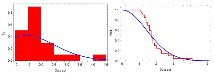
Our study aimed to compare ordered ranked set sampling with moving extremes ranked set sampling in the context of type Ⅱ censoring. We focused on deriving Bayesian estimations and predictions using the linear exponential model. This analysis included various loss functions, such as squared error, Al-Bayyati, and general entropy. To evaluate the efficiency of the estimators we produced, we assessed their mean squared error and relative absolute bias. Additionally, we provide Bayesian point and interval predictions for the ordered future lifetime, considering both squared error and general entropy loss functions. To ensure the accuracy and effectiveness of these estimation and prediction methods, we conducted numerical tests using Monte Carlo simulations. Finally, we illustrated these theoretical concepts with a practical example that utilized real-world medical data.
- ordered moving extremes ranked set sampling,
- Bayes estimation,
- squared error loss function,
- Al-Bayyati loss function,
- general entropy loss function,
- Bayesian prediction
Citation: Haidy A. Newer, Bader S Alanazi. Bayesian estimation and prediction for linear exponential models using ordered moving extremes ranked set sampling in medical data[J]. AIMS Mathematics, 2025, 10(1): 1162-1182. doi: 10.3934/math.2025055

Related Papers:

Abstract

Our study aimed to compare ordered ranked set sampling with moving extremes ranked set sampling in the context of type Ⅱ censoring. We focused on deriving Bayesian estimations and predictions using the linear exponential model. This analysis included various loss functions, such as squared error, Al-Bayyati, and general entropy. To evaluate the efficiency of the estimators we produced, we assessed their mean squared error and relative absolute bias. Additionally, we provide Bayesian point and interval predictions for the ordered future lifetime, considering both squared error and general entropy loss functions. To ensure the accuracy and effectiveness of these estimation and prediction methods, we conducted numerical tests using Monte Carlo simulations. Finally, we illustrated these theoretical concepts with a practical example that utilized real-world medical data.

References

[1]	W. Abu-Dayyeh, E. Al Sawi, Modified inference about the mean of the exponential distribution using moving extreme ranked set sampling, Stat. Papers, 50 (2009), 249–259. https://doi.org/10.1007/s00362-007-0072-5 doi: 10.1007/s00362-007-0072-5
[2]	A. Al-Omari, S. Al-Hadhrami, Bayes estimation of the mean of normal distribution using moving extreme ranked set sampling, Pak. J. Stat. Oper. Res., 8 (2012), 21–30. https://doi.org/10.18187/pjsor.v8i1.227 doi: 10.18187/pjsor.v8i1.227
[3]	M. T. Al-Odat, M. F. Al-Saleh, A variation of ranked set sampling, Journal of Applied Statistical Science, 10 (2001), 137–146.
[4]	M. F. Al-Saleh, S. A. Al-Hadhrami, Estimation of the mean of the exponential distribution using moving extremes ranked set sampling, Stat. Papers, 44 (2003), 367–382. https://doi.org/10.1007/s00362-003-0161-z doi: 10.1007/s00362-003-0161-z
[5]	M. F. Al-Saleh, S. A. Al-Hadrami, Parametric estimation for the location parameter for symmetric distributions using moving extremes ranked set sampling with application to trees data, Environmetrics, 14 (2003), 651–664. https://doi.org/10.1002/env.610 doi: 10.1002/env.610
[6]	H. S. Ali, M. M. Mohie El-Din, S. M. Elarishy, H. A. Newer, Inference for linear exponential distribution based on extreme ranked set sampling, Pak. J. Stat., 39 (2023), 415–432.
[7]	B. C. Arnold, N. Balakrishnan, H. N. Nagaraja, A first course in order statistics, Society for Industrial and Applied Mathematics, 2008. https://doi.org/10.1137/1.9780898719062
[8]	N. Balakrishnan, Permanents, order statistics, outliers, and robustness, Revista Matemática Complutense, 20 (2007), 7–107.
[9]	N. Balakrishnan, T. Li, Ordered ranked set samples and applications to inference, J. Stat. Plan. Infer., 138 (2008), 3512–3524. https://doi.org/10.1016/j.jspi.2005.08.050 doi: 10.1016/j.jspi.2005.08.050
[10]	J. O. Berger, Statistical decision theory and Bayesian analysis, New York, NY: Springer, 1985. https://doi.org/10.1007/978-1-4757-4286-2
[11]	S. Bhushan, A. Kumar, S. Shahab, S. A. Lone, S. A. Almutlak, Modified class of estimators using ranked set sampling, Mathematics, 10 (2022), 3921. https://doi.org/10.3390/math10213921 doi: 10.3390/math10213921
[12]	S. Bhushan, A. Kumar, S. A. Lone, On some novel classes of estimators under ranked set sampling, Alex. Eng. J., 61 (2022), 5465–5474. https://doi.org/10.1016/j.aej.2021.11.001 doi: 10.1016/j.aej.2021.11.001
[13]	S. Broadbent, Simple mortality rates, J. Royal Stat. Soc. C, 7 (1958), 86–95. https://doi.org/10.2307/2985310
[14]	R. Calabria, G. Pulcini, Point estimation under asymmetric loss functions for left-truncated exponential samples, Commun. Stat.-Theor. Meth., 25 (1996), 585–600. https://doi.org/10.1080/03610929608831715 doi: 10.1080/03610929608831715
[15]	P. P. Carbone, L. E. Kellerhouse, E. A. Gehan, Plasmacytic myeloma: a study of the relationship of survival to various clinical manifestations and anomalous protein type in 112 patients, The American Journal of Medicine, 42 (1967), 937–948. https://doi.org/10.1016/0002-9343(67)90074-5 doi: 10.1016/0002-9343(67)90074-5
[16]	G. Casella, R. Berger, Statistical inference, 2 Eds., New York: Chapman and Hall/CRC, 2024. https://doi.org/10.1201/9781003456285
[17]	Z. Chen, Z. Bai, B. K. Sinha, Ranked set sampling: theory and applications, New York: Springer, 2004. https://doi.org/10.1007/978-0-387-21664-5
[18]	W. Chen, M. Xie, M. Wu, Parametric estimation for the scale parameter for scale distributions using moving extremes ranked set sampling, Stat. Probabil. Lett., 83 (2013), 2060–2066. https://doi.org/10.1016/j.spl.2013.05.015 doi: 10.1016/j.spl.2013.05.015
[19]	W. Chen, M. Xie, M. Wu, Modified maximum likelihood estimator of scale parameter using moving extremes ranked set sampling, Commun. Stat.-Simul. Comput., 45 (2016), 2232–2240. https://doi.org/10.1080/03610918.2014.904520 doi: 10.1080/03610918.2014.904520
[20]	H. A. David, H. N. Nagaraja, Order statistics, 3 Eds., Hoboken: Wiley, 2003. https://doi.org/10.1002/0471722162
[21]	R. M. EL-Sagheer, M. S. Eliwa, K. M. Alqahtani, M. EL-Morshedy, A. Sajid, Asymmetric randomly censored mortality distribution: Bayesian framework and parametric bootstrap with application to COVID-19 data, J. Math., 2022 (2022), 8300753. https://doi.org/10.1155/2022/8300753 doi: 10.1155/2022/8300753
[22]	M. M. M. El-Din, M. S. Kotb, E. F. Abd-Elfattah, H. A. Newer, Bayesian inference and prediction of the Pareto distribution based on ordered ranked set sampling, Commun. Stat.-Theor. Meth., 46 (2017), 6264–6279. https://doi.org/10.1080/03610926.2015.1124118 doi: 10.1080/03610926.2015.1124118
[23]	M. M. M. El-Din, M. S. Kotb, H. A. Newer, Inference for linear exponential distribution based on record ranked set sampling, Journal of Statistics Applications & Probability, 10 (2021), 512–524. https://doi.org/10.18576/jsap/100219 doi: 10.18576/jsap/100219
[24]	M. M. M. El-Din, M. S. Kotb, H. A. Newer, Bayesian estimation and prediction of the Rayleigh distribution based on ordered ranked set sampling under type-Ⅱ doubly censored samples, Journal of Statistics Applications & Probability Letters, 8 (2021), 83–95. https://doi.org/10.18576/jsapl/080202 doi: 10.18576/jsapl/080202
[25]	M. M. M. El-Din, M. S. Kotb, H. A. Newer, Bayesian estimation and prediction for Pareto distribution based on ranked set sampling, Journal of Statistics Applications & Probability, 4 (2015), 1–11.
[26]	A. J. Gross, V. A. Clark, Survival distributions: reliability applications in the biomedical sciences, New York: Wiley, 1975.
[27]	C. D. Lai, M. Xie, Bathtub shaped failure rate life distributions, In: Stochastic ageing and dependence for reliability, New York, NY: Springer, 2006, 71–107. https://doi.org/10.1007/0-387-34232-X_3
[28]	C. D. Lai, M. Xie, D. N. P. Murthy, Bathtub-shaped failure rate life distributions, In: Handbook of statistics Vol. 20, Elsevier, 2001, 69–104. https://doi.org/10.1016/S0169-7161(01)20005-4
[29]	E. L. Lehmann, G. Casella, Theory of point estimation, 2 Eds., New York: Springer, 1998. https://doi.org/10.1007/b98854
[30]	G. A. McIntyre, A method for unbiased selective sampling. using ranked sets, Australian Journal of Agricultural Research, 3 (1952), 385–390. https://doi.org/10.1071/AR9520385 doi: 10.1071/AR9520385
[31]	H. A. Newer, M. M. M. El-Din, H. S. Ali, I. Al-Shbeil, W. Emam, Statistical inference for the Nadarajah-Haghighi distribution based on ranked set sampling with applications, AIMS Math., 8 (2023), 21572–21590. https://doi.org/10.3934/math.20231099 doi: 10.3934/math.20231099
[32]	T. Zhang, M. Xie, L. C. Tang, S. H. Ng, Reliability and modeling of systems integrated with firmware and hardware, Int. J. Reliab. Qual. Safety Eng., 12 (2005), 227–239. https://doi.org/10.1142/S021853930500180X doi: 10.1142/S021853930500180X

Reader Comments

Your name:*

Email:*
© 2025 the Author(s), licensee AIMS Press. This is an open access article distributed under the terms of the Creative Commons Attribution License (http://creativecommons.org/licenses/by/4.0)