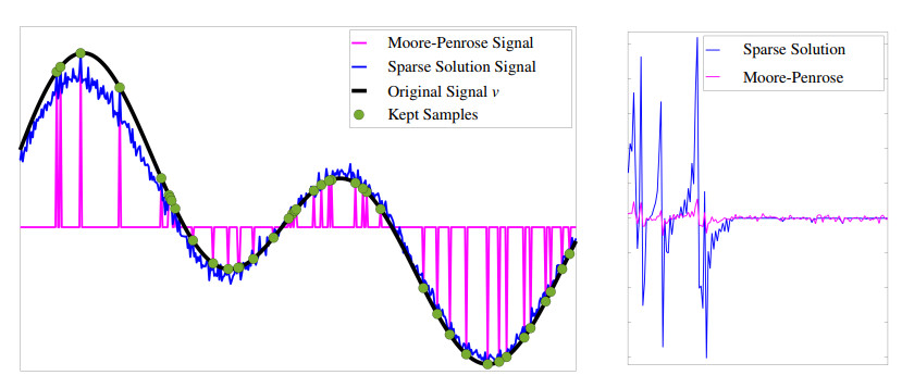
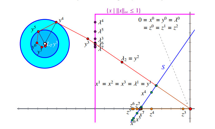
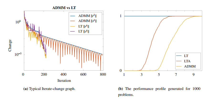
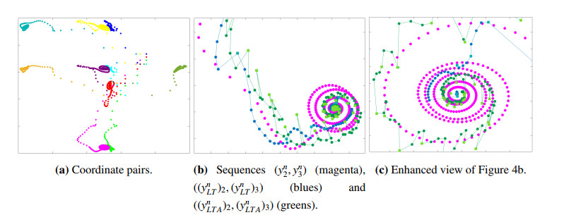
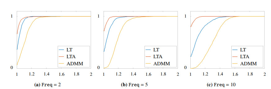
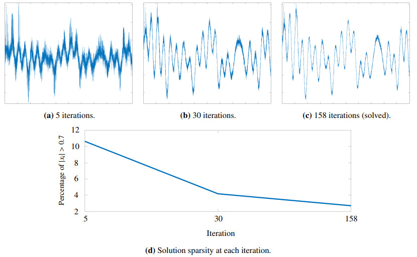
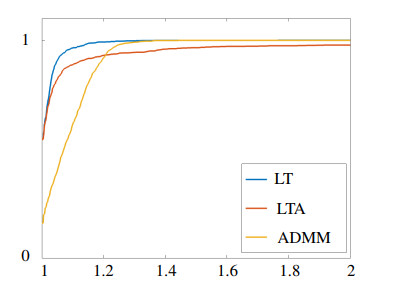
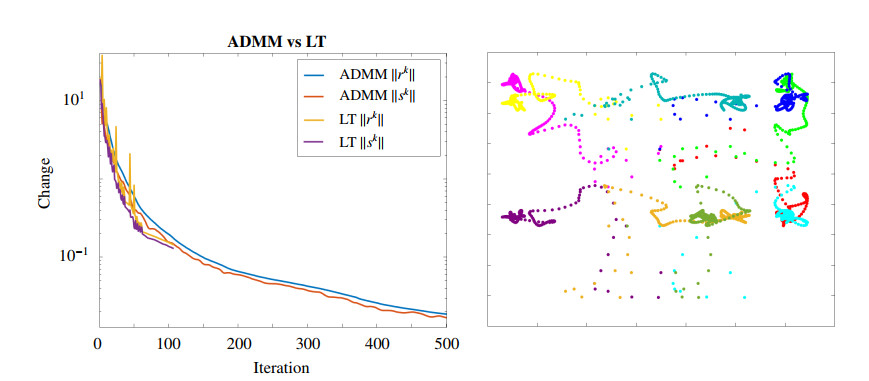
Practitioners employ operator splitting methods—such as alternating direction method of multipliers (ADMM) and its "dual" Douglas-Rachford method (DR)—to solve many kinds of optimization problems. We provide a gentle introduction to these algorithms, and illustrations of their duality-like relationship in the context of solving basis pursuit problems for audio signal recovery. Recently, researchers have used the dynamical systems associated with the iterates of splitting methods to motivate the development of schemes to improve performance. These developments include a class of methods that act by iteratively minimizing surrogates for a Lyapunov function for the dynamical system. An exemplar of this class is currently state-of-the-art for the feasibility problem of finding wavelets with special structure. Early experimental evidence has also suggested that, when implemented in a primal-dual (ADMM and DR) framework, this exemplar may provide improved performance for basis pursuit problems. We provide a reasonable way to compute the updates for this exemplar, and we study the application of this method to the aforementioned basis pursuit audio problems. We provide experimental results and visualizations of the dynamical system for the dual DR sequence. We observe that for highly structured problems with real data, the algorithmic behavior is noticeably different than for randomly generated problems.
Citation: Andrew Calcan, Scott B. Lindstrom. The ADMM algorithm for audio signal recovery and performance modification with the dual Douglas-Rachford dynamical system[J]. AIMS Mathematics, 2024, 9(6): 14640-14657. doi: 10.3934/math.2024712
Practitioners employ operator splitting methods—such as alternating direction method of multipliers (ADMM) and its "dual" Douglas-Rachford method (DR)—to solve many kinds of optimization problems. We provide a gentle introduction to these algorithms, and illustrations of their duality-like relationship in the context of solving basis pursuit problems for audio signal recovery. Recently, researchers have used the dynamical systems associated with the iterates of splitting methods to motivate the development of schemes to improve performance. These developments include a class of methods that act by iteratively minimizing surrogates for a Lyapunov function for the dynamical system. An exemplar of this class is currently state-of-the-art for the feasibility problem of finding wavelets with special structure. Early experimental evidence has also suggested that, when implemented in a primal-dual (ADMM and DR) framework, this exemplar may provide improved performance for basis pursuit problems. We provide a reasonable way to compute the updates for this exemplar, and we study the application of this method to the aforementioned basis pursuit audio problems. We provide experimental results and visualizations of the dynamical system for the dual DR sequence. We observe that for highly structured problems with real data, the algorithmic behavior is noticeably different than for randomly generated problems.

| [1] |
R. Arefidamghani, R. Behling, Y. Bello-Cruz, A. Iusem, L. Santos, The circumcentered-reflection method achieves better rates than alternating projections, Comput. Optim. Appl., 79 (2021), 507–530. http://dx.doi.org/10.1007/s10589-021-00275-6 doi: 10.1007/s10589-021-00275-6

|
| [2] |
H. Attouch, On the maximality of the sum of two maximal monotone operators, Nonlinear Anal.-Theor., 5 (1981), 143–147. http://dx.doi.org/10.1016/0362-546X(81)90039-0 doi: 10.1016/0362-546X(81)90039-0
|
| [3] | H. Bauschke, P. Combettes, Convex analysis and monotone operator theory in Hilbert spaces, Cham: Springer, 2 Eds., 2017. http://dx.doi.org/10.1007/978-3-319-48311-5 |
| [4] | H. Bauschke, H. Ouyang, X. Wang, On circumcenters of finite sets in Hilbert spaces, arXiv: 1807.02093. |
| [5] |
R. Behling, Y. Bello-Cruz, L. Santos, Circumcentering the Douglas-Rachford method, Numer. Algor., 78 (2018), 759–776. http://dx.doi.org/10.1007/s11075-017-0399-5 doi: 10.1007/s11075-017-0399-5
|
| [6] |
R. Behling, Y. Bello-Cruz, L. Santos, On the linear convergence of the circumcentered-reflection method, Oper. Res. Lett., 46 (2018), 159–162. http://dx.doi.org/10.1016/j.orl.2017.11.018 doi: 10.1016/j.orl.2017.11.018
|
| [7] |
R. Behling, Y. Bello-Cruz, L. Santos, On the circumcentered-reflection method for the convex feasibility problem, Numer. Algor., 86 (2021), 1475–1494. http://dx.doi.org/10.1007/s11075-020-00941-6 doi: 10.1007/s11075-020-00941-6
|
| [8] |
J. Benoist, The Douglas-Rachford algorithm for the case of the sphere and the line, J. Glob. Optim., 63 (2015), 363–380. http://dx.doi.org/10.1007/s10898-015-0296-1 doi: 10.1007/s10898-015-0296-1
|
| [9] | D. Bertsekas, Convex optimization theory, Melrose: Athena Scientific, 2009. |
| [10] | J. Borwein, A. Lewis, Convex analysis and nonlinear optimization: theory and examples, New York: Springer, 2 Eds., 2006. http://dx.doi.org/10.1007/978-0-387-31256-9 |
| [11] | S. Boyd, L. Vandenberghe, Convex optimisation, Cambridge: Cambridge University Press, 2004. http://dx.doi.org/10.1017/CBO9780511804441 |
| [12] | S. Boyd, N. Parikh, E. Chu, B. Peleato, J. Eckstein, Matlab scripts for alternating direction method of multipliers, 2011. Available from: https://web.stanford.edu/~boyd/papers/admm/. |
| [13] | S. Boyd, N. Parikh, E. Chu, B. Peleato, J. Eckstein, Distributed optimisation and statistical learning via the alternating direction method of multipliers, New York: Now Foundations and Trends, 2010. http://dx.doi.org/10.1561/2200000016 |
| [14] |
M. Dao, M. Tam, A Luapunov-type approach to convergence of the Douglas-Rachford algorithm, J. Glob. Optim., 73 (2019), 83–112. http://dx.doi.org/10.1007/s10898-018-0677-3 doi: 10.1007/s10898-018-0677-3
|
| [15] |
N. Dizon, J. Hogan, S. Lindstrom, Circumcentered reflections method for wavelet feasibility problems, ANZIAM J., 62 (2020), C98–C111. http://dx.doi.org/10.21914/anziamj.v62.16118 doi: 10.21914/anziamj.v62.16118
|
| [16] | N. Dizon, J. Hogan, S. Lindstrom, Centering projection methods for wavelet feasibility problems, In Current trends in analysis, its applications and computation, Cham: Birkhäuser, 2022. http://dx.doi.org/10.1007/978-3-030-87502-2_66 |
| [17] | Neil Dizon, J. A. Hogan, and Scott B. Lindstrom, Circumcentering reflection methods for nonconvex feasibility problems. Set-Valued Var. Anal., 30 (2022), 943–973. http://dx.doi.org/10.1007/s11228-021-00626-9 |
| [18] |
E. Dolan, J. Moré, Benchmarking optimisation software with performance profiles, Math. Program., 91 (2022), 201–213. http://dx.doi.org/10.1007/s101070100263 doi: 10.1007/s101070100263
|
| [19] | J. Eckstein, W. Yao, Understanding the convergence of the alternating direction method of multipliers: theoretical and computational perspectives, Pac. J. Optim., 11 (2015), 619–644. |
| [20] |
D. Gabay, Applications of the method of multipliers to variational inequalities, Studies in Mathematics and its Applications, 15 (1983), 299–331. http://dx.doi.org/10.1016/S0168-2024(08)70034-1 doi: 10.1016/S0168-2024(08)70034-1
|
| [21] |
O. Giladi, B. Rüffer, A Lyapunov function construction for a non-convex Douglas-Rachford iteration, J. Optim. Theory Appl., 180 (2019), 729–750. http://dx.doi.org/10.1007/s10957-018-1405-3 doi: 10.1007/s10957-018-1405-3
|
| [22] |
B. He, X. Yuan, On the O(1/n) convergence rate of the Douglas-Rachford alternating direction method, SIAM J. Numer. Anal., 50 (2012), 700–709. http://dx.doi.org/10.1137/110836936 doi: 10.1137/110836936
|
| [23] |
B. He, X. Yuan, On the convergence rate of Douglas-Rachford operator splitting method, Math. Program., 153 (2015), 715–722. http://dx.doi.org/10.1007/s10107-014-0805-x doi: 10.1007/s10107-014-0805-x
|
| [24] |
S. B. Lindstrom, Computable centering methods for spiralling algorithms and their duals with motivations from the theory of Lyapunov functions, Comput. Optim. Appl., 83 (2022), 999–1026. http://dx.doi.org/10.1007/s10589-022-00413-8 doi: 10.1007/s10589-022-00413-8
|
| [25] |
S. B. Lindstrom, B. Sims, Survey: sixty years of Douglas-Rachford, J. Aust. Math. Soc., 110 (2021), 333–370. http://dx.doi.org/10.1017/S1446788719000570 doi: 10.1017/S1446788719000570
|
| [26] |
P. Lions, B. Mercier, Splitting algorithms for the sum of two nonlinear operators, SIAM J. Numer. Anal., 16 (1979), 964–979. http://dx.doi.org/10.1137/0716071 doi: 10.1137/0716071
|
Figures(9) / Tables(2)

Andrew Calcan, Scott B. Lindstrom. The ADMM algorithm for audio signal recovery and performance modification with the dual Douglas-Rachford dynamical system[J]. AIMS Mathematics, 2024, 9(6): 14640-14657. doi: 10.3934/math.2024712


 DownLoad: