Novel categories of supra soft continuous maps via new soft operators

1.   Introduction

Many engineers and scientists have turned their attention to ambiguity or uncertainty modeling in order to extract the applicable information from uncertain data. Recently, scholars have presented a number of notions concerning uncertainty, e.g., fuzzy sets ^[1], intuitionistic fuzzy sets ^[2], rough sets ^[3,4], real valued interval mathematics ^[5], and so on. Pawlak ^[3] in 1982 pioneered rough set theory as a tool to help analyze the uncertainty in real-life problems. Generally, the objects in rough set theory could be categorized by using an equivalence relation based on the meaning of their properties (features). In ^[3], Pawlak replaced the ambiguous concept with two definite sets, i.e., lower approximation and upper approximation. This style of roughness of a universe set is built on equivalence classes generated by the associated equivalence relations. Many researchers have deduced that equivalence relations could not be used to solve real-life problems through the application of general rough set theory such as in ^[6,7,8,9].

In 1999, Molodtsov ^[10] submitted the first article on soft sets as a new method that can deal with uncertainties. The properties of these soft sets give a standardized framework for modeling ambiguity problems such as in decision making problems ^[11,12], diagnostic problems in medicine ^[13,14,15], the evaluation of nutrition systems ^[16] and problems in information systems ^[17]. Soft topological notions were defined in ^[18,19]. The notion of an ideal model of this type can be seen in ^[20], and there are many research studies concerned with the idealized versions of numerous rough set models. The effect or the advantage of employing an ideal version is reduction of the ambiguity of a concept in an uncertainty zone by shrinking the boundary region of roughness and enhancing the accuracy measure of roughness. As a result, using an ideal model is a great way to demystify the concept and define it precisely. Accordingly, many researchers have studied this theory by using ideals such as those in ^{[21,22,23,24]}.

Rough set theory and soft set theory are two different tools to deal with uncertainty. Apparently there is no direct connection between these two theories; however, efforts have been made to establish some kind of linkage ^[25,26]. The major criticism of rough set theory is that it lacks parametrization tools ^[27]. In order to make parametrization tools available in rough sets a major step was taken by Feng et al. ^[28]. They introduced the concept of soft rough sets, where instead of equivalence classes parametrized subsets of a set serve the purpose of finding lower and upper approximations of a subset. In doing so, some unusual situations may occur. For example upper approximation of a non-empty set may be empty. Upper approximation of a subset X may not contain the set X. These situations do not occur in classical rough set theory. Moreover, the soft rough set model must be reduced to be able to get a true decision of any real-life problem. Therefore, the authors of ^[29] modified the concept of soft rough sets to solve the previous problems. In order to strengthen the concept of soft rough sets and solve the previous problems more accurately than the method given in ^[29], new approaches that apply the ideals are presented here.

In this paper, we submit two novel approaches for soft rough sets that apply the ideals, as defined in ^[30]. These new approaches are extensions of soft rough sets approaches that have been introduced in ^[28,29]. The main characteristics of the recent approaches are investigated, and comparisons between our methods and previous ones are applied. We illustrate that the soft rough approximations ^[28] constitute a special case of the current approximations in the first method in Definition 3.2, and that the soft rough approximations ^[29] constitute a special case of the current approximations in the second method in Definition 3.5. Moreover, we prove that our second method is the best one since it produces smaller boundary regions and higher accuracy values than our first method and those introduced in ^[28,29]. Therefore, this method is more applicable to real-life problems and can be used to determine the vagueness of the data. Furthermore, new soft rough sets that were developed by using two ideals, called soft bi-ideal rough sets, are presented. These soft approximations are discussed from the perspective of two different methods. The properties and results of these soft bi-ideal rough sets are provided. The relationships between these two approximations and the previous ones are discussed. However, comparisons between the last two methods are presented and we discuss which of them is the best. Finally, two medical applications are provided to demonstrate the significance of adopting ideals in the current techniques. In the proposed applications, we illustrate that our techniques reduce boundary regions and improve the accuracy measure of the sets more than the approaches presented in ^[28,29], which means that the current techniques allow the medical staff to classify patients successfully in terms of influenza infection (see ^[31,32]) (first application) and heart attacks (see ^[33]) (second application). That helps doctors to make the best decision.

2.   Preliminaries

The aim of this section is to illustrate the basic concepts and properties of rough sets and soft sets which are needed in the sequel.

Definition 2.1. ^[3] If $X$ is a universal set of objects, $R$ is an equivalence relation on $X$ and $[x]_R$ is the proposed equivalence class containing $x$. Then for $A \subseteq X$, the lower approximation, the upper approximation, the boundary region and the accuracy measure of $A$ are defined respectively, as follows:

Clearly, $0\leq ACC(A)\leq 1.$ $A$ is a crisp set if $\underline{Aprox}(A) = \overline{Aprox}(A);$ otherwise, $A$ is called a rough set.

Definition 2.2. ^[3] The membership relations of an element $x \in X$ to a rough set $A \subseteq X$ are defined by:

Definition 2.3. ^[3] For two rough subsets $A, B \subseteq X$, the inclusion relations are defined as follows:

Proposition 2.1. ^[3] Let $A, B$ be two subsets of $X$. The following is a list of the main characterizations of the approximation operators defined in Definition 2.1,

$(\mathrm{L}_1)$ $\underline{Aprox}(A^c) = [\overline{Aprox}(A)]^c;$

$(\mathrm{L}_2)$ $\underline{Aprox}(X) = X;$

$(\mathrm{L}_3)$ $\underline{Aprox}(\phi) = \phi;$

$(\mathrm{L}_4)$ $\underline{Aprox}(A)\subseteq A;$

$(\mathrm{L}_5)$ $A\subseteq B\Rightarrow \underline{Aprox}(A)\subseteq\underline{Aprox}(B) \ (A\underline{\subseteq} B);$

$(\mathrm{L}_6)$ $\underline{Aprox}[\underline{Aprox}(A)] = \underline{Aprox}(A);$

$(\mathrm{L}_7)$ $\underline{Aprox}(A\cap B) = \underline{Aprox}(A)\cap \underline{Aprox}(B);$

$(\mathrm{L}_8)$ $\underline{Aprox}(A)\cup \underline{Aprox}(B)\subseteq\underline{Aprox}(A\cup B);$

$(\mathrm{L}_9)$ $\underline{Aprox}[\overline{Aprox}(A)] = \overline{Aprox}(A);$

$(\mathrm{U}_1)$ $\overline{Aprox}(A^c) = [\underline{Aprox}(A)]^c;$

$(\mathrm{U}_2)$ $\overline{Aprox}(X) = X;$

$(\mathrm{U}_3)$ $\overline{Aprox}(\phi) = \phi;$

$(\mathrm{U}_4)$ $A\subseteq\overline{Aprox}(A);$

$(\mathrm{U}_5)$ $A\subseteq B\Rightarrow \overline{Aprox}(A)\subseteq\overline{Aprox}(B) \ (A\overline{\subseteq} B);$

$(\mathrm{U}_6)$ $\overline{Aprox}[\overline{Aprox}(A)] = \overline{Aprox}(A);$

$(\mathrm{U}_7)$ $\overline{Aprox}(A\cap B)\subseteq \overline{Aprox}(A)\cap \overline{Aprox}(B);$

$(\mathrm{U}_8)$ $\overline{Aprox}(A)\cup \overline{Aprox}(B) = \overline{Aprox}(A\cup B);$

$(\mathrm{U}_9)$ $\overline{Aprox}[\underline{Aprox}(A)] = \underline{Aprox}(A)$.

Definition 2.4. ^[10] Let $X$ be the universal set, $E\neq\phi$ a family of parameters which represent attributes or decision variables and $H\subseteq E$. A pair $(F, H)$ is said to be a soft set of $X$ if $F$ is a mapping from $H$ to the power set of $X,$ i.e., $F: H \longrightarrow P(X).$ Therefore, a soft set is a set of parameterized elements from $X.$ To each $e\in H$, $F(e)$ is a subset of $X$, which is usually named the set of e-approximate elements of $(F, H)$. Also, $F(e)$ can be regarded as a mapping $F(e):X\longrightarrow \{0, 1\}$, and then $F(e)(x) = 1$ is equivalent to $x\in F(e)$ for $x\in X$.

Definition 2.5. ^[28] Let $\mathbf{S} = (F, E)$ be a soft set of a universe $X$. Then, $P = (X, \mathbf{S})$ is said to be a soft approximation space. For any subset $A$ of $X$, the soft P-lower approximation, the soft P-upper approximation and the soft P-boundary region are defined respectively, as follows:

Theorem 2.1. ^[28] Let $P = (X, \mathbf{S})$ be a soft approximation space. Then, the approximations defined in Definition 2.5 satisfy the conditions of the properties $\mathrm{L}_3, \mathrm{L}_5, \mathrm{L}_6, \mathrm{L}_8, \mathrm{L}_9, \mathrm{U}_3, \mathrm{U}_5, \mathrm{U}_7, \mathit{\text{and}}\mathrm{U}_8$ in Proposition 2.1.

Definition 2.6. ^[28] Let $\mathbf{S} = (F, E)$ be a soft set of $X.$ If $\bigcup_{e\in E}F(e) = X$, then $\mathbf{S}$ is called a full soft set.

Definition 2.7. ^[28] Let $\mathbf{S} = (F, E)$ be a soft set over $X.$ If for any $e_1, e_2\in E$, there is $e_3\in E$ such that $F(e_3) = F(e_1)\cap F(e_2)$ whenever $F(e_1)\cap F(e_2)\neq\phi,$ then $\mathbf{S}$ is called an intersecting complete soft set.

Definition 2.8. ^[29] Let $P = (X, \mathbf{S})$ be a soft approximation space where $\mathbf{S} = (F, E)$ is a soft set of $X$, and $A \subseteq X$. Based on P, the soft lower approximation, the soft upper approximation and the soft boundary region are defined respectively, as follows:

Definition 2.9. ^[29] Let $P = (X, \mathbf{S})$ be a soft approximation space. Based on P, one can deduce that the degree of crispness of any $A \subseteq X$ is given by the rough measures $Acc_{apr}(A)$ and $Acc_{\mathbf{S}R}(A)$ that are respectively given by

Obviously, $0\leq Acc_{apr}(A)\leq1$ and $0\leq Acc_{\mathbf{S}R}(A)\leq1.$

Theorem 2.2. ^[29] Let $P = (X, \mathbf{S})$ be a soft approximation space. Then, the approximations defined in Definition 2.8 satisfy the conditions of the properties $\mathrm{L}_1$, $\mathrm{L}_3$–$\mathrm{L}_6$, $\mathrm{L}_8$ and $\mathrm{U}_1, \mathrm{U}_2$, $\mathrm{U}_4$–$\mathrm{U}_7$ in Proposition 2.1.

Definition 2.10. ^[29] Let $\mathbf{S} = (F, E)$ be a full soft set of $X$, and let $P = (X, \mathbf{S})$ be a soft approximation space. Then, $A\subseteq X$ is referred to as follows:

(1) A totally $\mathbf{S}R$-definable ($\mathbf{S}R$-exact) set if $\underline{\mathbf{S}R}(A) = \overline{\mathbf{S}R}(A) = A$.

(2) An internally $\mathbf{S}R$-definable set if $\underline{\mathbf{S}R}(A) = A \ \text{ and } \ \overline{\mathbf{S}R}(A)\neq A$.

(3) An externally $\mathbf{S}R$-definable set if $\underline{\mathbf{S}R}(A)\neq A\text{ and } \overline{\mathbf{S}R}(A) = A$.

(4) A totally $\mathbf{S}R$-rough set if $\underline{\mathbf{S}R}(A) \neq A \neq \ \overline{\mathbf{S}R}(A)$.

Definition 2.11. ^[29] Let $P = (X, \mathbf{S})$ be a soft approximation space where $\mathbf{S} = (F, E)$ is a soft set of $X$. Let $A\subseteq X$ and $x\in X.$ The $\mathbf{S}R$-membership relations, denoted by $\underline{\in}_{\mathbf{S}R}, \overline{\in}_{\mathbf{S}R}$ are given by

Definition 2.12. ^[30] Let $X$ be a universal set. Then, a non-empty family $\mathcal{L}$ of subsets of $X$ is said to be an ideal on $X$ if it fulfills the following conditions.

(1) If $A\in \mathcal{L}$ and $B\subseteq A,$ then $B\in \mathcal{L}.$

(2) If $A, B\in \mathcal{L},$ then $A\cup B\in \mathcal{L}.$

Definition 2.13. ^[22] Let $\mathcal{L}_1, \mathcal{L}_2$ be two ideals on a non-empty set $X$. Then, the family of subsets from $\mathcal{L}_1, \mathcal{L}_2$ is denoted as $< \mathcal{L}_1, \mathcal{L}_2 >$ and defined by

Proposition 2.2. ^[22] Let $\mathcal{L}_1, \mathcal{L}_2$ be two ideals on a non-empty set $X$ and $A, B\subseteq X$. Then, the collection $< \mathcal{L}_1, \mathcal{L}_2 >$ has the following proprieties:

(1) $< \mathcal{L}_1, \mathcal{L}_2 > \neq\phi;$

(2) $A\in \ < \mathcal{L}_1, \mathcal{L}_2 > , \ B \subseteq A \ \Rightarrow \ \ B\in \ < \mathcal{L}_1, \mathcal{L}_2 > ;$

(3) $A, B \ \in \ < \mathcal{L}_1, \mathcal{L}_2 > \ \ \Rightarrow \ \ A\cup B\in \ < \mathcal{L}_1, \mathcal{L}_2 > .$

3.   New types of soft rough set approximations through the use of ideals

In this section, we will generalize the soft rough set theory by using the ideal notion. Also, we will present some properties of soft ideal rough approximation operators and introduce two new soft rough set models based on the ideals, which constitutes an improvement of the models by Feng et al. ^[28] and Alkhazaleh and Marei ^[29].

3.1.   First style of soft rough set approximations

Definition 3.1. Let $\mathbf{S} = (F, E)$ be a soft set of a universal set $X$ and $\mathcal{L}$ an ideal on $X.$ Then, $P = (X, \mathbf{S}, \mathcal{L})$ is said to be a soft ideal approximation space. For any subset $A$ of $X$, the soft P-lower approximation and the soft P-upper approximation, i.e., $(apr_\mathcal{L})_*(A)$ and $(apr_\mathcal{L})^*(A)$, are defined respectively, as follows:

Proposition 3.1. Let $P = (X, \mathbf{S}, \mathcal{L})$ be a soft ideal approximation space and $A, B\subseteq X.$ Then, the conditions of the following properties are fulfilled.

(1) $(apr_\mathcal{L})_*(\phi) = \cup\{F(e):e\in E, F(e)\in \mathcal{L}\}$ and $(apr_\mathcal{L})^*(\phi) = \phi;$

(2) $(apr_\mathcal{L})_*(X) = \cup\{F(e), e\in E\}$ and $(apr_\mathcal{L})^*(X) = \cup\{F(e):e\in E, F(e)\notin \mathcal{L}\}$;

(3) $A\subseteq B\Rightarrow (apr_\mathcal{L})_*(A)\subseteq (apr_\mathcal{L})_*(B);$

(4) $A\subseteq B\Rightarrow (apr_\mathcal{L})^*(A)\subseteq (apr_\mathcal{L})^*(B);$

(5) $(apr_\mathcal{L})_*[(apr_\mathcal{L})_*(A)] = (apr_\mathcal{L})_*(A);$

(6) $(apr_\mathcal{L})^*(A)\subseteq (apr_\mathcal{L})^*[(apr_\mathcal{L})^*(A)];$

(7) $(apr_\mathcal{L})^*(A) \subseteq (apr_\mathcal{L})_*[(apr_\mathcal{L})^*(A)];$

(8) $(apr_\mathcal{L})_*(A\cap B)\subseteq (apr_\mathcal{L})_*(A)\cap(apr_\mathcal{L})_*(B);$

(9) $(apr_\mathcal{L})_*(A)\cup(apr_\mathcal{L})_*(B)\subseteq(apr_\mathcal{L})_*(A\cup B);$

(10) $(apr_\mathcal{L})^*(A\cap B)\subseteq (apr_\mathcal{L})^*(A)\cap(apr_\mathcal{L})^*(B);$

(11) $(apr_\mathcal{L})^*(A)\cup(apr_\mathcal{L})^*(B) = (apr_\mathcal{L})^*(A\cup B).$

Proof. (1), (2) Straightforward from Definition 3.1.

(3) Let $A\subseteq B$ and $x\in(apr_\mathcal{L})_*(A) = \{x\in X:\exists e\in E, x\in F(e), F(e) \cap A^c\in \mathcal{L}\}.$ Then, $x\in F(e), F(e) \cap A^c\in \mathcal{L}$ for some $e\in E.$ But, $A\subseteq B$ and $\mathcal{L}$ is an ideal, so $x\in F(e), F(e) \cap B^c\in \mathcal{L}.$ Thus, $x\in(apr_\mathcal{L})_*(B).$ Hence, $(apr_\mathcal{L})_*(A)\subseteq (apr_\mathcal{L})_*(B).$

(4) Let $A\subseteq B$ and $x\in (apr_\mathcal{L})^*(A) = \{x\in X:\exists e\in E, x\in F(e), F(e) \cap A\notin \mathcal{L}\}.$ Then, $x\in F(e), F(e) \cap A\notin \mathcal{L}$ for some $e\in E.$ But, $A\subseteq B$ and $\mathcal{L}$ is an ideal, so $x\in F(e), F(e) \cap B^c\in \mathcal{L}.$ Therefore, $(apr_\mathcal{L})^*(A)\subseteq (apr_\mathcal{L})^*(B).$

(5) Let $x\in (apr_\mathcal{L})_*(A) = \{x\in X:\exists e\in E, x\in F(e), F(e) \cap A^c\in \mathcal{L}\}.$ Therefor for some $e\in E:x\in F(e),$ we have that $F(e) \cap A^c\in \mathcal{L}.$ So, $F(e)\subseteq (apr_\mathcal{L})_*(A)$ which means that $F(e)\cap [(apr_\mathcal{L})_*(A)]^c = \phi\in \mathcal{L}.$ Hence, $x\in (apr_\mathcal{L})_*[(apr_\mathcal{L})_*(A)].$

Conversely, let $x\notin (apr_\mathcal{L})_*(A)$. Then, for all $e\in E:x\in F(e),$ we have that $F(e) \cap A^c\notin \mathcal{L}.$ Thus, $\exists y\in F(e), y\in A^c, \{y\}\notin \mathcal{L}.$ So, $y\notin (apr_\mathcal{L})_*(A)$ and $\{y\}\notin \mathcal{L},$ which means that $\{y\}\cap[(apr_\mathcal{L})_*(A)]^c\notin \mathcal{L}$ and, for all $e\in E:y\in F(e),$ we have that $F(e) \cap [(apr_\mathcal{L})_*(A)]^c\notin \mathcal{L}.$ Hence, $x\notin (apr_\mathcal{L})_*[(apr_\mathcal{L})_*(A)].$

(6) Let $x\in (apr_\mathcal{L})^*(A) = \{x\in X:\exists e\in E, x\in F(e), F(e) \cap A\notin \mathcal{L}\}.$ Therefore, for some $e\in E:x\in F(e)$ we have that $F(e) \cap A\notin \mathcal{L}.$ So, $F(e)\subseteq (apr_\mathcal{L})^*(A)$ which means that $F(e)\cap(apr_\mathcal{L})^*(A) = F(e)\notin\mathcal{L}.$ Thus, $x\in (apr_\mathcal{L})^*[(apr_\mathcal{L})^*(A)].$ Hence, $(apr_\mathcal{L})^*(A)\subseteq(apr_\mathcal{L})^*[(apr_\mathcal{L})^*(A)].$

(7) Let $x\notin (apr_\mathcal{L})_*[(apr_\mathcal{L})^*(A)] = \{x\in X:\exists e\in E, x\in F(e), F(e) \cap [(apr_\mathcal{L})^*(A)]^c\in \mathcal{L}\}$. Then, for all $e\in E:x\in F(e)$ we have that $F(e) \cap [(apr_\mathcal{L})^*(A)]^c\notin \mathcal{L}.$ Thus, $\exists y\in F(e), y\notin(apr_\mathcal{L})^*(A).$ So, for some $e\in E:y\in F(e),$ we have that $F(e) \cap A\in \mathcal{L}$ thus, $x\in F(e)$ and $F(e) \cap A\in \mathcal{L}.$ Therefore, $x\notin (apr_\mathcal{L})^*(A).$ Hence, $(apr_\mathcal{L})^*(A)\subseteq (apr_\mathcal{L})_*[(apr_\mathcal{L})^*(A)].$

(8) Let $x\in (apr_\mathcal{L})_*(A\cap B) = \{x\in X:\exists e\in E, x\in F(e), F(e) \cap (A^c\cup B^c)\in \mathcal{L}\}.$ Thus, $\exists F(e)$ such that $x\in F(e)$ and $F(e) \cap (A^c\cup B^c)\in \mathcal{L}.$ Therefore, $x\in F(e), F(e) \cap A^c\in \mathcal{L}$ and $x\in F(e), F(e) \cap B^c\in \mathcal{L}.$ Consequently, $x\in (apr_\mathcal{L})_*(A)$ and $x\in (apr_\mathcal{L})_*(B).$ Hence, $(apr_\mathcal{L})_*(A\cap B)\subseteq (apr_\mathcal{L})_*(A)\cap(apr_\mathcal{L})_*(B).$

(9) Let, $x\notin (apr_\mathcal{L})_*(A\cup B).$ Thus, $\forall e\in E:x\in F(e),$ we have that $F(e) \cap (A^c\cap B^c)\notin \mathcal{L}.$ Therefore, $\forall e\in E:x\in F(e),$ we have that $F(e) \cap A^c\notin \mathcal{L}$ and $F(e) \cap B^c\notin \mathcal{L}.$ Consequently, $x\notin (apr_\mathcal{L})_*(A)$ and $x\notin (apr_\mathcal{L})_*(B).$ Hence, $(apr_\mathcal{L})_*(A)\cup(apr_\mathcal{L})_*(B)\subseteq(apr_\mathcal{L})_*(A\cup B).$

(10) Similar to part (7).

(11)

□

Remark 3.1. Let $P = (X, \mathbf{S}, \mathcal{L})$ be a soft ideal approximation space and $A, B\subseteq X.$ Then, the following example ensures that

(1) $(apr_\mathcal{L})_*(X)\neq X, (apr_\mathcal{L})^*(X)\neq X$ and $(apr_\mathcal{L})_*(\phi)\neq \phi,$

(2) $(apr_\mathcal{L})_*(A)\nsubseteq A,$ $A\nsubseteq (apr_\mathcal{L})_*(A)$ and $(apr_\mathcal{L})^*(A)\nsubseteq A,$ $A\nsubseteq (apr_\mathcal{L})^*(A),$

(3) $(apr_\mathcal{L})_*(A)\subseteq (apr_\mathcal{L})_*(B)\nRightarrow A\subseteq B$ and $(apr_\mathcal{L})^*(A)\subseteq (apr_\mathcal{L})^*(B)\nRightarrow A\subseteq B,$

(4) $(apr_\mathcal{L})^*(A)\neq(apr_\mathcal{L})^*[(apr_\mathcal{L})^*(A)]$ and $(apr_\mathcal{L})^*(A) \neq (apr_\mathcal{L})_*[(apr_\mathcal{L})^*(A)],$

(5) $(apr_\mathcal{L})^*(A)\nsubseteq[(apr_\mathcal{L})_*(A^c)]^c$ and $(apr_\mathcal{L})^*(A)\nsupseteq[(apr_\mathcal{L})_*(A^c)]^c,$

(6) $(apr_\mathcal{L})_*(A) \nsubseteq (apr_\mathcal{L})^*[(apr_\mathcal{L})_*(A)]$ and $(apr_\mathcal{L})_*(A) \nsupseteq(apr_\mathcal{L})^*[(apr_\mathcal{L})_*(A)],$

(7) $(apr_\mathcal{L})_*(A\cap B)\neq(apr_\mathcal{L})_*(A)\cap (apr_\mathcal{L})_*(B)$ and $(apr_\mathcal{L})^*(A\cap B)\neq(apr_\mathcal{L})^*(A)\cap (apr_\mathcal{L})^*(B).$

Example 3.1. Let $X = \{x_1, x_2, x_3, x_4, x_5, x_6\}, E = \{e_1, e_2, e_3, e_4, e_5, e_6, e_7, e_8\}$, $F: E\longrightarrow P(X),$ $\mathbf{S} = (F, E)$ be a soft set over $X,$ as given in Table 1, and $\mathcal{L} = \{\phi, \{x_1\}, \{x_6\}, \{x_1, x_6\}\}.$ From Table 1, we can deduce that

Hence, we obtain the following results:

(1) From Proposition 3.1 part (2), we have that $(apr_\mathcal{L})_*(X) = (apr_\mathcal{L})^*(X) = \{x_1, x_2, x_3, x_5, x_6\}\neq X.$ Also, $(apr_\mathcal{L})_*(\phi) = \{x\in X:\exists e\in E, x\in F(e), F(e) \cap X\in \mathcal{L}\} = \{x_1, x_6\}\neq \phi.$

(2) Let $A = \{x_3, x_4\}.$ Then, $(apr_\mathcal{L})_*(A) = \{x_1, x_6\}$. Hence, $(apr_\mathcal{L})_*(A)\nsubseteq A$ and $A\nsubseteq (apr_\mathcal{L})_*(A).$

(3) Let $A = \{x_1, x_2, x_4\};$ then, $(apr_\mathcal{L})^*(A) = \{x\in X:\exists e\in E, x\in F(e), F(e) \cap \{x_1, x_2, x_4\}\notin \mathcal{L}\} = \{x_1, x_2, x_3, x_5, x_6\}$. Hence, $(apr_\mathcal{L})^*(A)\nsubseteq A$ and $A\nsubseteq (apr_\mathcal{L})^*(A).$

(4) Let $A = \{x_1, x_2, x_5\}, B = \{x_1, x_2, x_4\}.$ Then, $(apr_\mathcal{L})_*(A) = \{x_1, x_2, x_5, x_6\}$ and $(apr_\mathcal{L})_*(B) = \{x_1, x_2, x_6\}.$ So, $(apr_\mathcal{L})_*(B)\subseteq(apr_\mathcal{L})_*(A)$ but $B\nsubseteq A.$ Also, if $A = \{x_4, x_5, x_6\}$, $B = \{x_3, x_5, x_6\}.$ Then, $(apr_\mathcal{L})^*(A) = \{x_1, x_2, x_3, x_5\}$ and $(apr_\mathcal{L})^*(B) = \{x_1, x_2, x_3, x_5, x_6\}.$ So, $(apr_\mathcal{L})^*(A)\subseteq(apr_\mathcal{L})^*(B)$ but $A\nsubseteq B.$

(5) If $A = \{x_4, x_5\},$ then $(apr_\mathcal{L})^*(A) = \{x_1, x_2, x_3, x_5\}$. So, $(apr_\mathcal{L})^*[(apr_\mathcal{L})^*(A)] = \{x_1, x_2, x_3, x_5, x_6\}.$ Hence, $(apr_\mathcal{L})^*(A) \neq (apr_\mathcal{L})^*[(apr_\mathcal{L})^*(A)].$ Also, $(apr_\mathcal{L})_*[(apr_\mathcal{L})^*(A)] = \{x_1, x_2, x_3, x_5, x_6\}.$ Hence, $(apr_\mathcal{L})^*(A) \neq (apr_\mathcal{L})_*[(apr_\mathcal{L})^*(A)].$

(6) Let $A = \{x_1, x_2, x_3, x_5, x_6\}.$ Then, $(apr_\mathcal{L})^*(A) = \{x_1, x_2, x_3, x_5, x_6\}$ but $[(apr_\mathcal{L})_*(A^c)]^c = \{x_2, x_3, x_4, x_5\}.$ Therefore, $(apr_\mathcal{L})^*(A)\nsubseteq[(apr_\mathcal{L})_*(A^c)]^c$ and $(apr_\mathcal{L})^*(A)\nsupseteq[(apr_\mathcal{L})_*(A^c)]^c.$

(7) Let $A = \{x_1, x_6\}.$ Then, $(apr_\mathcal{L})_*(A) = \{x_1, x_6\}$. So, $(apr_\mathcal{L})^*[(apr_\mathcal{L})_*(A)] = \phi.$ Hence, $(apr_\mathcal{L})_*(A) \nsubseteq(apr_\mathcal{L})^*[(apr_\mathcal{L})_*(A)].$ Also, if $A = \{x_2, x_3, x_4\}$ then $(apr_\mathcal{L})_*(A) = \{x_1, x_2, x_3, x_6\}$. So, $(apr_\mathcal{L})^*[(apr_\mathcal{L})_*(A)] = \{x_1, x_2, x_3, x_5, x_6\}.$ Therefore, $(apr_\mathcal{L})_*(A) \nsupseteq(apr_\mathcal{L})^*[(apr_\mathcal{L})_*(A)].$

(8) Consider that $\mathcal{L}=\{\phi, \{x_1\}, \{x_5\}, \{x_1, x_5\}\}.$ If $A=\{x_1, x_2, x_3, x_5\}$ and $B=\{x_1, x_6\},$ then $(apr_\mathcal{L})_*(A)\cap (apr_\mathcal{L})_*(B)=\{x_1, x_2, x_3, x_5\}\cap \{x_1, x_6\}=\{x_1\}$ but $(apr_\mathcal{L})_*(A\cap B)=(apr_\mathcal{L})_*(\{x_1\})=\phi.$ Also, if $A=\{x_2, x_3\}$ and $B=\{x_4, x_5, x_6\},$ then $(apr_\mathcal{L})^*(A)\cap (apr_\mathcal{L})^*(B)=\{x_1, x_2, x_3, x_5, x_6\}\cap \{x_1, x_2, x_3, x_6\}=\{x_1, x_2, x_3, x_6\}$ but $(apr_\mathcal{L})^*(A\cap B)(apr_\mathcal{L})^*(\phi)=\phi.$

Definition 3.2. Let $\mathbf{S} = (F, E)$ be a soft set of the universal set $X$ and $\mathcal{L}$ an ideal on $X.$ Then, $P = (X, \mathbf{S}, \mathcal{L})$ is said to be a soft ideal approximation space. For any subset $A$ of $X$, the soft P-lower approximation and the soft P-upper approximation, i.e., $\underline{apr_\mathcal{L}}(A)$ and $\overline{apr_\mathcal{L}}(A)$, are defined respectively, as follows:

Proposition 3.2. Let $P = (X, \mathbf{S}, \mathcal{L})$ be a soft ideal approximation space and $A, B\subseteq X.$ Then, the following conditions of the properties are fulfilled.

(1) $\underline{apr_\mathcal{L}}(\phi) = \overline{apr_\mathcal{L}}(\phi) = \phi$ and $\overline{apr_\mathcal{L}}(X) = X;$

(2) $\underline{apr_\mathcal{L}}(A)\subseteq A \subseteq \overline{apr_\mathcal{L}}(A);$

(3) $A\subseteq B\Rightarrow \underline{apr_\mathcal{L}}(A)\subseteq \underline{apr_\mathcal{L}}(B)$ and $\overline{apr_\mathcal{L}}(A)\subseteq \overline{apr_\mathcal{L}}(B);$

(4) $\underline{apr_\mathcal{L}}[\underline{apr_\mathcal{L}}(A)] = \underline{apr_\mathcal{L}}(A)$ and $\overline{apr_\mathcal{L}}[\overline{apr_\mathcal{L}}(A)]\supseteq\overline{apr_\mathcal{L}}(A);$

(5) $\underline{apr_\mathcal{L}}[\overline{apr_\mathcal{L}}(A)] = \overline{apr_\mathcal{L}}(A)$ and $\underline{apr_\mathcal{L}}(A)\subseteq\overline{apr_\mathcal{L}}[\underline{apr_\mathcal{L}}(A)];$

(6) $\underline{apr_\mathcal{L}}(A\cap B)\subseteq \underline{apr_\mathcal{L}}(A)\cap\underline{apr_\mathcal{L}}(B)$ and $\underline{apr_\mathcal{L}}(A)\cup\underline{apr_\mathcal{L}}(B)\subseteq\underline{apr_\mathcal{L}}(A\cup B);$

(7) $\overline{apr_\mathcal{L}}(A\cap B)\subseteq \overline{apr_\mathcal{L}}(A)\cap\overline{apr_\mathcal{L}}(B)$ and $\overline{apr_\mathcal{L}}(A)\cup\overline{apr_\mathcal{L}}(B) = \overline{apr_\mathcal{L}}(A\cup B).$

Proof. Straightforward. □

Remark 3.2. Any one can define different ideals to obtain an example that is analogous to Example 3.1 to prove that the inclusion in Proposition 3.2 parts (2) and (4)–(8) could not be changed to the equality.

Definition 3.3. Let $P = (X, \mathbf{S}, \mathcal{L})$ be a soft ideal approximation space and $\mathbf{S} = (F, E)$ a soft set of $X$; also, let $A \subseteq X$. Then, the soft $apr_\mathcal{L}$-boundary region $Bnd_{apr_\mathcal{L}}(A)$ and the soft $apr_\mathcal{L}$-accuracy measure $Acc_{apr_\mathcal{L}}(A)$ are defined respectively, as follows:

3.2.   Second style of soft rough set approximations

Definition 3.4. Let $P = (X, \mathbf{S}, \mathcal{L})$ be a soft ideal approximation space in which $\mathbf{S} = (F, E)$ is a soft set over a universal set $X$; also, let there be an ideal $\mathcal{L}$ on $X$ and $A \subseteq X$. For any subset $A$ of $X$, the lower approximation and the upper approximation, $(\mathbf{S}R_\mathcal{L})_*(A)$ and $(\mathbf{S}R_\mathcal{L})^*(A)$, are defined respectively, as follows:

Proposition 3.3. Let $P = (X, \mathbf{S}, \mathcal{L})$ be a soft ideal approximation space $A, B\subseteq X.$ Then, the following conditions of the properties are fulfilled.

(1) $(\mathbf{S}R_\mathcal{L})_*(A^c) = [(\mathbf{S}R_\mathcal{L})^*(A)]^c;$

(2) $A\subseteq B\Rightarrow (\mathbf{S}R_\mathcal{L})_*(A)\subseteq (\mathbf{S}R_\mathcal{L})_*(B);$

(3) $A\subseteq B\Rightarrow (\mathbf{S}R_\mathcal{L})^*(A)\subseteq (\mathbf{S}R_\mathcal{L})^*(B);$

(4) $(\mathbf{S}R_\mathcal{L})_*[(\mathbf{S}R_\mathcal{L})_*(A)] = (\mathbf{S}R_\mathcal{L})_*(A);$

(5) $(\mathbf{S}R_\mathcal{L})^*[(\mathbf{S}R_\mathcal{L})^*(A)] = (\mathbf{S}R_\mathcal{L})^*(A);$

(6) $(\mathbf{S}R_\mathcal{L})_*(A\cap B)\subseteq (\mathbf{S}R_\mathcal{L})_*(A)\cap(\mathbf{S}R_\mathcal{L})_*(B);$

(7) $(\mathbf{S}R_\mathcal{L})_*(A)\cup(\mathbf{S}R_\mathcal{L})_*(B)\subseteq(\mathbf{S}R_\mathcal{L})_*(A\cup B);$

(8) $(\mathbf{S}R_\mathcal{L})^*(A\cap B)\subseteq (\mathbf{S}R_\mathcal{L})^*(A)\cap(\mathbf{S}R_\mathcal{L})^*(B);$

(9) $(\mathbf{S}R_\mathcal{L})^*(A)\cup(\mathbf{S}R_\mathcal{L})^*(B)\subseteq(\mathbf{S}R_\mathcal{L})^*(A\cup B).$

Proof. (1) $[(\mathbf{S}R_\mathcal{L})^*(A)]^c = [((\mathbf{S}R_\mathcal{L})_*(A^c))^c]^c = (\mathbf{S}R_\mathcal{L})_*(A^c)$.

(2) Let $A\subseteq B$ and $x\in(\mathbf{S}R_\mathcal{L})_*(A) = \cup\{F(e), e\in E:F(e) \cap A^c\in \mathcal{L}\}.$ Then, $\exists F(e)$ such that $x\in F(e),$ where $F(e) \cap A^c\in \mathcal{L}.$ But, $A\subseteq B;$ thus, $x\in F(e), F(e) \cap B^c\in \mathcal{L}.$ Hence, $x\in(\mathbf{S}R_\mathcal{L})_*(B)$ and $(\mathbf{S}R_\mathcal{L})_*(A)\subseteq (\mathbf{S}R_\mathcal{L})_*(B).$

(3) Let $A\subseteq B.$ Thus, $B^c\subseteq A^c$ and then $(\mathbf{S}R_\mathcal{L})_*(B^c)\subseteq (\mathbf{S}R_\mathcal{L})_*(A^c).$ Hence, $[(\mathbf{S}R_\mathcal{L})_*(A^c)]^c\subseteq [(\mathbf{S}R_\mathcal{L})_*(B^c)]^c.$ Consequently, $(\mathbf{S}R_\mathcal{L})^*(A)\subseteq (\mathbf{S}R_\mathcal{L})^*(B).$

(4) Let $x\in (\mathbf{S}R_\mathcal{L})_*(A) = \cup\{F(e), e\in E:F(e) \cap A^c\in \mathcal{L}\}.$ Therefor for some $e\in E:x\in F(e),$ we have that $F(e) \cap A^c\in \mathcal{L}.$ So, $F(e)\subseteq (\mathbf{S}R_\mathcal{L})_*(A)$ which means that $F(e)\cap [(\mathbf{S}R_\mathcal{L})_*(A)]^c = \phi\in \mathcal{L}.$ Hence, $x\in (\mathbf{S}R_\mathcal{L})_*[(\mathbf{S}R_\mathcal{L})_*(A)].$

Conversely, let $x\notin (\mathbf{S}R_\mathcal{L})_*(A)$. Then, for all $e\in E:x\in F(e),$ we have that $F(e) \cap A^c\notin \mathcal{L}.$ Thus, $\exists y\in F(e), y\in A^c, \{y\}\notin \mathcal{L}.$ So, $y\notin (\mathbf{S}R_\mathcal{L})_*(A), \{y\}\notin \mathcal{L},$ which means that $\{y\}\cap[(\mathbf{S}R_\mathcal{L})_*(A)]^c\notin \mathcal{L}$ and, for all $e\in E:y\in F(e),$ we have that $F(e) \cap [(\mathbf{S}R_\mathcal{L})_*(A)]^c\notin \mathcal{L}.$ Hence, $x\notin (\mathbf{S}R_\mathcal{L})_*[(\mathbf{S}R_\mathcal{L})_*(A)].$

(5) It follows directly by putting $A = A^c$ in part (4) and using part (1).

(6) Let $x\in (\mathbf{S}R_\mathcal{L})_*(A\cap B) = \cup\{F(e), e\in E:F(e) \cap (A^c\cup B^c)\in \mathcal{L}\}.$ Then, $\exists F(e)$ such that $x\in F(e),$ where $F(e) \cap (A^c\cup B^c)\in \mathcal{L}.$ Therefore, $x\in F(e), F(e) \cap A^c\in \mathcal{L}$ and $x\in F(e), F(e) \cap B^c\in \mathcal{L}.$ Consequently, $x\in (\mathbf{S}R_\mathcal{L})_*(A)$ and $x\in (\mathbf{S}R_\mathcal{L})_*(B).$ Hence, $(\mathbf{S}R_\mathcal{L})_*(A\cap B)\subseteq (\mathbf{S}R_\mathcal{L})_*(A)\cap(\mathbf{S}R_\mathcal{L})_*(B).$

(7) Let $x\notin (\mathbf{S}R_\mathcal{L})_*(A\cup B) = \cup\{F(e), e\in E:F(e) \cap (A^c\cap B^c)\in \mathcal{L}\}.$ Then, $\forall e\in E:x\in F(e),$ we have that $F(e) \cap (A^c\cap B^c)\notin \mathcal{L}.$ Therefore, $\forall e\in E:x\in F(e),$ we have that $F(e) \cap A^c\notin \mathcal{L}$ and $F(e) \cap B^c\notin \mathcal{L}.$ Consequently, $x\notin (\mathbf{S}R_\mathcal{L})_*(A)$ and $x\notin (\mathbf{S}R_\mathcal{L})_*(B).$ Hence, $(\mathbf{S}R_\mathcal{L})_*(A)\cup(\mathbf{S}R_\mathcal{L})_*(B)\subseteq(\mathbf{S}R_\mathcal{L})_*(A\cup B).$

(8) It follows directly by putting $A = A^c, B = B^c$ in part (6) and using part (1).

(9) It follows directly by putting $A = A^c, B = B^c$ in part (7) and using part (1). □

Remark 3.3. Let $P = (X, \mathbf{S}, \mathcal{L})$ be a soft ideal approximation space and $A, B\subseteq X.$ Then, the next examples ensure that

(1) $(\mathbf{S}R_\mathcal{L})_*(X)\neq X$ and $(\mathbf{S}R_\mathcal{L})^*(\phi)\neq \phi;$

(2) $(\mathbf{S}R_\mathcal{L})_*(\phi)\neq \phi$ and $(\mathbf{S}R_\mathcal{L})^*(X)\neq X;$

(3) $(\mathbf{S}R_\mathcal{L})_*(A)\nsubseteq A,$$A\nsubseteq (\mathbf{S}R_\mathcal{L})_*(A)$ and $(\mathbf{S}R_\mathcal{L})^*(A)\nsubseteq A,$ $A\nsubseteq (\mathbf{S}R_\mathcal{L})^*(A);$

(4) $(\mathbf{S}R_\mathcal{L})_*(A)\subseteq (\mathbf{S}R_\mathcal{L})_*(B)\nRightarrow A\subseteq B$ and $(\mathbf{S}R_\mathcal{L})^*(A)\subseteq (\mathbf{S}R_\mathcal{L})^*(B)\nRightarrow A\subseteq B;$

(5) $(\mathbf{S}R_\mathcal{L})^*(A) \nsubseteq (\mathbf{S}R_\mathcal{L})_*[(\mathbf{S}R_\mathcal{L})^*(A)]$ and $(\mathbf{S}R_\mathcal{L})^*(A) \nsupseteq (\mathbf{S}R_\mathcal{L})_*[(\mathbf{S}R_\mathcal{L})^*(A)];$

(6) $(\mathbf{S}R_\mathcal{L})_*(A) \nsubseteq (\mathbf{S}R_\mathcal{L})^*[(\mathbf{S}R_\mathcal{L})_*(A)]$ and $(\mathbf{S}R_\mathcal{L})_*(A) \nsupseteq (\mathbf{S}R_\mathcal{L})^*[(\mathbf{S}R_\mathcal{L})_*(A)];$

(7) $(\mathbf{S}R_\mathcal{L})_*(A\cap B)\neq(\mathbf{S}R_\mathcal{L})_*(A)\cap (\mathbf{S}R_\mathcal{L})_*(B)$ and $(\mathbf{S}R_\mathcal{L})^*(A\cup B)\neq(\mathbf{S}R_\mathcal{L})^*(A)\cup (\mathbf{S}R_\mathcal{L})^*(B).$

Example 3.2. Let $X = \{x_1, x_2, x_3, x_4, x_5, x_6\}, E = \{e_1, e_2, e_3, e_4, e_5\},$ $F: E\longrightarrow P(X),$ $\mathbf{S} = (F, E)$ be a soft set of $X,$ as given in Table 2, and $\mathcal{L} = \{\phi, \{x_1\}, \{x_6\}, \{x_1, x_6\}\}.$ From Table 2, we can deduce that

Hence, we obtain the following results:

(1) $(\mathbf{S}R_\mathcal{L})_*(X) = \cup\{F(e), e\in E:F(e) \cap X^c\in \mathcal{L})\} = \{x_1, x_2, x_3, x_5, x_6\}\neq X.$ Then, $(\mathbf{S}R_\mathcal{L})^*(\phi) = [(\mathbf{S}R_\mathcal{L})_*(X)]^c = \{x_4\}\neq \phi.$

(2) $(\mathbf{S}R_\mathcal{L})_*(\phi)=\cup\{F(e), e\in E:F(e) \cap \phi^c\in \mathcal{L})\}=\{x_1, x_6\}\neq \phi.$ Then, $(\mathbf{S}R_\mathcal{L})^*(X)= [(\mathbf{S}R_\mathcal{L})_*(\phi)]^c=\{x_2, x_3, x_4, x_5\}\neq X.$

(3) Let $A = \{x_4\}.$ Then, $(\mathbf{S}R_\mathcal{L})_*(A) = \{x_1, x_6\}$. Hence. $(\mathbf{S}R_\mathcal{L})_*(A)\nsubseteq A$ and $A\nsubseteq (\mathbf{S}R_\mathcal{L})_*(A).$

(4) From part (3), if $A = \{x_1, x_2, x_3, x_5, x_6\},$ then $(\mathbf{S}R_\mathcal{L})^*(A) = \{x_2, x_3, x_4, x_5\}$. Hence, $(\mathbf{S}R_\mathcal{L})^*(A)\nsubseteq A$ and $A\nsubseteq (\mathbf{S}R_\mathcal{L})^*(A).$

(5) Let $A = \{x_1, x_2, x_3\}$ and $B = \{x_1, x_2, x_4\}.$ Then, $(\mathbf{S}R_\mathcal{L})_*(A) = \{x_1, x_2, x_3, x_6\}$ and $(\mathbf{S}R_\mathcal{L})_*(B) = \{x_1, x_6\}.$ So, $(\mathbf{S}R_\mathcal{L})_*(B)\subseteq(\mathbf{S}R_\mathcal{L})_*(A),$ but $B\nsubseteq A.$ Also, if $A = \{x_4, x_5, x_6\}$ and $B = \{x_3, x_5, x_6\},$ then $(\mathbf{S}R_\mathcal{L})^*(A) = \{x_4, x_5\}$ and $(\mathbf{S}R_\mathcal{L})^*(B) = \{x_2, x_3, x_4, x_5\}.$ So, $(\mathbf{S}R_\mathcal{L})^*(A)\subseteq(\mathbf{S}R_\mathcal{L})^*(B)$ but $A\nsubseteq B.$

(6) From part (4), if $A = \{x_1, x_2, x_3, x_5, x_6\},$ then $(\mathbf{S}R_\mathcal{L})^*(A) = \{x_2, x_3, x_4, x_5\}$. So, $(\mathbf{S}R_\mathcal{L})_*[(\mathbf{S}R_\mathcal{L})^*(A)] = X.$ Hence, $(\mathbf{S}R_\mathcal{L})^*(A) \nsupseteq (\mathbf{S}R_\mathcal{L})_*[(\mathbf{S}R_\mathcal{L})^*(A)].$

(7) From part (6), if $A = \{x_1, x_2, x_3, x_5, x_6\},$ then $(\mathbf{S}R_\mathcal{L})_*(A) = A$ but $(\mathbf{S}R_\mathcal{L})^*[(\mathbf{S}R_\mathcal{L})_*(A)] = (\mathbf{S}R_\mathcal{L})^*(A) = \{x_2, x_3, x_4, x_5\}$. Hence, $(\mathbf{S}R_\mathcal{L})_*(A) \nsubseteq (\mathbf{S}R_\mathcal{L})^*[(\mathbf{S}R_\mathcal{L})_*(A)]$ and $(\mathbf{S}R_\mathcal{L})_*(A) \nsupseteq (\mathbf{S}R_\mathcal{L})^*[(\mathbf{S}R_\mathcal{L})_*(A)].$

(8) Consider that $\mathcal{L} = \{\phi, \{x_4\}, \{x_6\}, \{x_4, x_6\}\}$ and $A = \{x_1, x_2, x_5\}.$ Then, $(\mathbf{S}R_\mathcal{L})^*(A) = \{x_1, x_2, x_4, x_5, x_6\}$. So, $(\mathbf{S}R_\mathcal{L})_*[(\mathbf{S}R_\mathcal{L})^*(A)] = \{x_1, x_6\}.$ Hence, $(\mathbf{S}R_\mathcal{L})^*(A) \nsubseteq (\mathbf{S}R_\mathcal{L})_*[(\mathbf{S}R_\mathcal{L})^*(A)].$

(9) Consider that $\mathcal{L} = \{\phi, \{x_4\}, \{x_5\}, \{x_4, x_5\}\}.$ If $A = \{x_1, x_2, x_3, x_5\}$ and $B = \{x_1, x_6\},$ then $(\mathbf{S}R_\mathcal{L})_*(A)\cap (\mathbf{S}R_\mathcal{L})_*(B) = \{x_1, x_2, x_3, x_5\}\cap \{x_1, x_6\} = \{x_1\}$ but $(\mathbf{S}R_\mathcal{L})_*(A\cap B) = (\mathbf{S}R_\mathcal{L})_*(\{x_1\}) = \phi.$ Also, if $A = \{x_2, x_3\}$ and $B = \{x_4, x_5, x_6\},$ then $(\mathbf{S}R_\mathcal{L})^*(A)\cup (\mathbf{S}R_\mathcal{L})^*(B) = \{x_2, x_3, x_4, x_5\}\cup \{x_4, x_6\} = \{x_2, x_3, x_4, x_5, x_6\}$ but $(\mathbf{S}R_\mathcal{L})^*(A\cup B) = X.$

Definition 3.5. Let $P = (X, \mathbf{S}, \mathcal{L})$ be a soft ideal approximation space in which $\mathbf{S} = (F, E)$ is a soft set of $X$; also, an ideal $\mathcal{L}$ is given and $A \subseteq X$. Based on P, the lower approximation and the upper approximation, $\underline{\mathbf{S}R_\mathcal{L}}(A)$ and $\overline{\mathbf{S}R_\mathcal{L}}(A)$, are defined respectively, as follows:

Definition 3.6. Let $P = (X, \mathbf{S}, \mathcal{L})$ be a soft ideal approximation space and $\mathbf{S} = (F, E)$ a soft set of $X$ and let $A \subseteq X$. Then, the soft $\mathbf{S}R_\mathcal{L}$-boundary region $Bnd_{\mathbf{S}R_\mathcal{L}}(A)$ and the soft $\mathbf{S}R_\mathcal{L}$-accuracy measure $Acc_{\mathbf{S}R_\mathcal{L}}(A)$ are defined respectively by:

Proposition 3.4. Let $P = (X, \mathbf{S}, \mathcal{L})$ be a soft ideal approximation space and $A, B\subseteq X.$ Then, the following conditions of the properties are fulfilled.

(1) $\underline{\mathbf{S}R_\mathcal{L}}(\phi) = \phi$ and $\overline{\mathbf{S}R_\mathcal{L}}(X) = X;$

(2) $\underline{\mathbf{S}R_\mathcal{L}}(A)\subseteq A \subseteq \overline{\mathbf{S}R_\mathcal{L}}(A);$

(3) $\underline{\mathbf{S}R_\mathcal{L}}(A^c) = [\overline{\mathbf{S}R_\mathcal{L}}(A)]^c$ and $\overline{\mathbf{S}R_\mathcal{L}}(A^c) = [\underline{\mathbf{S}R_\mathcal{L}}(A)]^c;$

(4) $A\subseteq B\Rightarrow \underline{\mathbf{S}R_\mathcal{L}}(A)\subseteq \underline{\mathbf{S}R_\mathcal{L}}(B)$ and $\overline{\mathbf{S}R_\mathcal{L}}(A)\subseteq \overline{\mathbf{S}R_\mathcal{L}}(B);$

(5) $\underline{\mathbf{S}R_\mathcal{L}}[\underline{\mathbf{S}R_\mathcal{L}}(A)] = \underline{\mathbf{S}R_\mathcal{L}}(A)$ and $\overline{\mathbf{S}R_\mathcal{L}}[\overline{\mathbf{S}R_\mathcal{L}}(A)] = \overline{\mathbf{S}R_\mathcal{L}}(A);$

(6) $\underline{\mathbf{S}R_\mathcal{L}}[\overline{\mathbf{S}R_\mathcal{L}}(A)]\subseteq\overline{\mathbf{S}R_\mathcal{L}}(A)$ and $\underline{\mathbf{S}R_\mathcal{L}}(A)\subseteq\overline{\mathbf{S}R_\mathcal{L}}[\underline{\mathbf{S}R_\mathcal{L}}(A)];$

(7) $\underline{\mathbf{S}R_\mathcal{L}}(A\cap B)\subseteq \underline{\mathbf{S}R_\mathcal{L}}(A)\cap\underline{\mathbf{S}R_\mathcal{L}}(B)$ and $\underline{\mathbf{S}R_\mathcal{L}}(A)\cup\underline{\mathbf{S}R_\mathcal{L}}(B)\subseteq\underline{\mathbf{S}R_\mathcal{L}}(A\cup B);$

(8) $\overline{\mathbf{S}R_\mathcal{L}}(A\cap B)\subseteq \overline{\mathbf{S}R_\mathcal{L}}(A)\cap\overline{\mathbf{S}R_\mathcal{L}}(B)$ and $\overline{\mathbf{S}R_\mathcal{L}}(A)\cup\overline{\mathbf{S}R_\mathcal{L}}(B)\subseteq\overline{\mathbf{S}R_\mathcal{L}}(A\cup B).$

Proof. Straightforward. □

Remark 3.4. Any one can define different ideals to obtain an example that is analogous to Example 3.2 to prove that the inclusion in Proposition 3.4 parts (2), (4) and (6)–(8) could not be changed to the equality.

In what follows, Table 3 summarizes the differences between the proposed properties of the two styles.

Corollary 3.1. Let $P = (X, \mathbf{S}, \mathcal{L})$ be a soft ideal approximation space and $A\subseteq X.$ Then,

Proof. Straightforward from Definitions 2.5, 2.8, 3.2 and 3.5. □

Theorem 3.1. Let $\mathbf{S} = (F, E)$ be a full soft set of $X$, $P = (X, \mathbf{S}, \mathcal{L})$ be a soft ideal approximation space and $A\subseteq X.$ Then,

(1) $\underline{apr}(A)\subseteq\underline{apr_\mathcal{L}}(A) = \underline{\mathbf{S}R_\mathcal{L}}(A) \subseteq A\subseteq\overline{\mathbf{S}R_\mathcal{L}}(A)\subseteq\overline{apr_\mathcal{L}}(A)\subseteq\overline{apr}(A);$

(2) $\underline{apr}(A)=\underline{\mathbf{S}R}(A)\subseteq\underline{\mathbf{S}R_\mathcal{L}}(A)\subseteq A\subseteq\overline{\mathbf{S}R_\mathcal{L}}(A)\subseteq\overline{\mathbf{S}R}(A)\subseteq\overline{apr}(A);$

(3) $Bnd_{\mathbf{S}R_\mathcal{L}}(A)\subseteq Bnd_{apr_\mathcal{L}}(A)\subseteq Bnd_{apr}(A)$ and $Bnd_{\mathbf{S}R_\mathcal{L}}(A)\subseteq Bnd_{\mathbf{S}R}(A)\subseteq Bnd_{apr}(A);$

(4) $Acc_{\mathbf{S}R_\mathcal{L}}(A)\geq Acc_{apr_\mathcal{L}}(A)\geq Acc_{apr}(A)$ and $Acc_{\mathbf{S}R_\mathcal{L}}(A)\geq Acc_{\mathbf{S}R}(A)\geq Acc_{apr}(A).$

Proof.

(1) By Corollary 3.1 and Proposition 3.4, we have that $\underline{apr}(A)\subseteq\underline{apr_\mathcal{L}}(A)\subseteq\underline{\mathbf{S}R_\mathcal{L}}(A) \subseteq A\subseteq\overline{\mathbf{S}R_\mathcal{L}}(A).$ To prove that $\overline{\mathbf{S}R_\mathcal{L}}(A)\subseteq\overline{apr_\mathcal{L}}(A),$ let $x\notin\overline{apr_\mathcal{L}}(A) = A\cup\{x\in X:\exists e\in E, x\in F(e), F(e) \cap A\notin \mathcal{L} \}.$ Then, $x\notin A$ and for all $e\in E; x\in F(e)$ we get that $F(e) \cap A\in \mathcal{L}.$ Thus, $x\notin A$ and $x\in(\mathbf{S}R_\mathcal{L})_*(A^c).$ That is, $x\notin A$ and $x\notin[(\mathbf{S}R_\mathcal{L})_*(A^c)]^c.$ Hence, $x\notin\overline{\mathbf{S}R_\mathcal{L}}(A).$ It follows that $\overline{\mathbf{S}R_\mathcal{L}}(A)\subseteq\overline{apr_\mathcal{L}}(A).$ To prove that $\overline{apr_\mathcal{L}}(A)\subseteq\overline{apr}(A),$ let $x\notin\overline{apr}(A) = \{x\in X:\exists e\in E, [x\in F(e), F(e) \cap A\ne \phi]\}.$ Then, for all $e\in E:x\in F(e)$ we have that $F(e) \cap A = \phi,$ which means that $F(e)\subseteq A^c.$ Thus, $x\notin A$ and $x\notin(apr_\mathcal{L})^*(A).$ Therefore, $x\notin\overline{apr_\mathcal{L}}(A).$ Hence, $\overline{apr_\mathcal{L}}(A)\subseteq\overline{apr}(A).$

(2) The proof is similar to that of part (1).

(3), (4) It is immediately obtained by applying parts (1) and (2). □

Remark 3.5. According to Theorem 3.1, the second style described in Definition 3.5 is the best technique to enhance approximations and increase the accuracy measure, which means that the vagueness/uncertainty is decreased by this style more than the other styles given in Definition 3.2, Definition 2.5 in ^[28] and Definition 2.8 in ^[29]. Hence, a decision made according to the calculations of the style in Definition 3.5 is more applicable based on the decrease to the upper approximations and the increase to the lower approximations; thus, we get a higher accuracy value than the accuracy values given by the other styles discussed in ^[28,29]. Consider the following as a special case:

(1) If $\mathcal{L} = \phi$ and $\mathbf{S}$ is a full soft set, then Definition 3.2 is consistent with the previous Definition 2.5 in ^[28].

(2) If $\mathcal{L} = \phi,$ then Definition 3.5 is consistent with the previous definition in ^[29].

4.   Modified soft rough concepts via ideals

In this section, we redefine some soft rough concepts as modified soft rough concepts by utilizing ideals. Comparisons between the present ideal soft rough concepts and the previous soft rough concepts in ^[28,29] are presented. Finally, some examples are used to explain the current definitions.

Definition 4.1. Let $\mathbf{S} = (F, E)$ be a full soft set of $X$ and $P = (X, \mathbf{S}, \mathcal{L})$ be a soft ideal approximation space. Then, $A\subseteq X$ is referred to as follows:

(1) A totally $\mathbf{S}R_\mathcal{L}$ (resp. $apr_\mathcal{L})$-definable set if $\underline{\mathbf{S}R_\mathcal{L}}(A) = \overline{\mathbf{S}R_\mathcal{L}}(A) = A$ (resp. $\underline{apr_\mathcal{L}}(A) = \overline{apr_\mathcal{L}}(A) = A)$.

(2) An internally $\mathbf{S}R_\mathcal{L}$ (resp. $apr_\mathcal{L})$-definable set if $\underline{\mathbf{S}R_\mathcal{L}}(A) = A, \ \overline{\mathbf{S}R_\mathcal{L}}(A)\neq A$ (resp. $\underline{apr_\mathcal{L}}(A) = A, \ \overline{apr_\mathcal{L}}(A)\neq A)$.

(3) An externally $\mathbf{S}R_\mathcal{L}$ (resp. $apr_\mathcal{L})$-definable set if $\underline{\mathbf{S}R_\mathcal{L}}(A)\neq A, \ \overline{\mathbf{S}R_\mathcal{L}}(A) = A$ (resp. $\underline{apr_\mathcal{L}}(A)\neq A, \ \overline{apr_\mathcal{L}}(A) = A)$.

(4) A totally $\mathbf{S}R_\mathcal{L}$ (resp. $apr_\mathcal{L})$-rough set if $\underline{\mathbf{S}R_\mathcal{L}}(A)\neq A \neq \overline{\mathbf{S}R_\mathcal{L}}(A)$ (resp. $\underline{apr_\mathcal{L}}(A)\neq A \neq \overline{apr_\mathcal{L}}(A)$.

Definition 4.2. Let $\mathbf{S} = (F, E)$ be a full soft set of $X$ and $P = (X, \mathbf{S})$ a soft approximation space. Then, $A\subseteq X$ is referred to as follows:

(1) A totally $apr$-definable set if $\underline{apr}(A) = \overline{apr}(A) = A$.

(2) An internally $apr$-definable set if $\underline{apr}(A) = A\text{ and }\overline{apr}(A)\neq A$.

(3) An externally $apr$-definable set if $\underline{apr}(A)\neq A\text{ and }\overline{apr}(A) = A$.

(4) A totally $apr$ -rough set if $\underline{apr}(A)\neq A \neq \overline{apr}(A)$.

Remark 4.1. From Definitions 2.10, 4.1 and 4.2 and by using Theorem 3.1, we have the following diagrams:

(1)

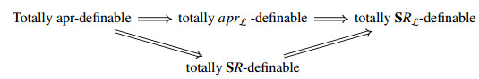
(2)

The following example explains how the implications in the previous diagrams are not reversible.

Example 4.1. Let $X = \{x_1, x_2, x_3, x_4, x_5, x_6\}, E = \{e_1, e_2, e_3, e_4, e_5, e6, e7, e8\}$, $F: E\longrightarrow P(X),$ and $\mathbf{S} = (F, E)$ be a soft set of $X$ as given in Table 3. From Table 4, we can deduce that

Hence, we obtain the following results:

(1) Consider that $\mathcal{L} = \{\phi, \{x_2\}, \{x_4\}, \{x_2, x_4\}\}.$ If $A = \{x_1, x_3, x_6\},$ then $(\mathbf{S}R_\mathcal{L})^*(A) = \phi$. So, $\overline{\mathbf{S}R_\mathcal{L}}(A) = A\cup(\mathbf{S}R_\mathcal{L})^*(A) = A\cup\phi = A.$ Also, $(\mathbf{S}R_\mathcal{L})_*(A) = \{x_1, x_3, x_4, x_6\}$. So, $\underline{\mathbf{S}R_\mathcal{L}}(A) = A\cap(\mathbf{S}R_\mathcal{L})_*(A) = \{x_1, x_3, x_6\} = A.$ Hence, $A$ is a totally $\mathbf{S}R_\mathcal{L}$-definable set. But $\overline{apr_\mathcal{L}}(A) = \overline{\mathbf{S}R}(A) = X\neq A.$ Therefore, $A$ is neither totally $apr_\mathcal{L}$ -definable nor totally $\mathbf{S}R$-definable set.

(2) Consider that $\mathcal{L} = \{\phi, \{x_1\}, \{x_2\}, \{x_3\}, \{x_1, x_2\}, \{x_1, x_3\}, \{x_2, x_3\}, \{x_1, x_2, x_3\}\}.$ If $A = \{x_1, x_2\},$ then $\underline{apr_\mathcal{L}}(A) = \overline{apr_\mathcal{L}}(A) = A.$ Thus, $A$ is a totally $apr_\mathcal{L}$-definable set. But $\overline{apr}(A) = X\neq A.$ Therefore, $A$ is not a totally $apr$-definable set. Also, if $A = \{x_1, x_4, x_6\},$ then $\underline{\mathbf{S}R}(A) = \overline{\mathbf{S}R}(A) = A.$ Therefore, $A$ is a totally $\mathbf{S}R$-definable set. But $\overline{apr}(A) = X\neq A.$ Hence, $A$ is not a totally $apr$-definable set.

(3) From part (1), if $A = \{x_1, x_3, x_6\},$ then $\underline{\mathbf{S}R}(A) = \{x_6\}\neq A$ and $\overline{\mathbf{S}R}(A) = X\neq A.$ Thus, $A$ is a totally $\mathbf{S}R$-rough set. But $\underline{\mathbf{S}R_\mathcal{L}}(A) = \overline{\mathbf{S}R_\mathcal{L}}(A) = A.$ So, $A$ is not a totally $\mathbf{S}R_\mathcal{L}$-rough set.

(4) From part (2), if $A = \{x_1, x_2\},$ then $\underline{apr}(A) = \phi\neq A$ and $\overline{apr}(A) = X\neq A.$ So, $A$ is a totally $apr$-rough set. But $\underline{apr_\mathcal{L}}(A) = \overline{apr_\mathcal{L}}(A) = A.$ Thus, $A$ is not a totally $apr_\mathcal{L}$-rough set.

(5) Let $A = \{x_4, x_5, x_6\}.$ Then, $\underline{apr}(A) = \{x_6\}\neq A$ and $\overline{apr}(A) = X\neq A.$ So, $A$ is a totally $apr$-rough set. But $\overline{\mathbf{S}R}(A) = A.$ Therefore, $A$ is not a totally $\mathbf{S}R$-rough set. Note that $A$ is an externally $\mathbf{S}R$-definable set.

(6) Consider that $\mathcal{L} = \{\phi, \{x_2\}, \{x_4\}, \{x_2, x_4\}\}$ and $A = \{x_1, x_2, x_4\}.$ Then, $\underline{apr_\mathcal{L}}(A) = \phi\neq A$ and $\overline{apr_\mathcal{L}}(A) = X\neq A.$ So, $A$ is a totally $apr_\mathcal{L}$-rough set. But $\overline{\mathbf{S}R_\mathcal{L}}(A) = A.$ Therefore, $A$ is not a totally $\mathbf{S}R_\mathcal{L}$-rough set. Also, $A$ is an externally $\mathbf{S}R_\mathcal{L}$-definable set. If $A = \{x_1, x_3, x_5, x_6\},$ then $\underline{apr_\mathcal{L}}(A) = A$ and $\overline{apr_\mathcal{L}}(A) = X\neq A.$ Hence, $A$ is an internally $apr_\mathcal{L}$-definable set.

Proposition 4.1. Let $P = (X, \mathbf{S}, \mathcal{L})$ be a soft ideal approximation space in which $\mathbf{S} = (F, E)$ is a soft set of $X$ and $A\subseteq X.$ Then, the following holds:

(1) $A$ is a totally $\mathbf{S}R_\mathcal{L}$-definable set iff $Acc_{\mathbf{S}R_\mathcal{L}}(A) = 1.$

(2) $A$ is a totally $apr_\mathcal{L}$-definable set iff $Acc_{apr_\mathcal{L}}(A) = 1.$

(3) $A$ is a totally $apr$-definable set $\Longrightarrow Acc_{apr}(A) = 1.$

Proof.

(1) Let $A$ be a totally $\mathbf{S}R_\mathcal{L}$-definable set. Then, $\underline{\mathbf{S}R_\mathcal{L}}(A) = \overline{\mathbf{S}R_\mathcal{L}}(A) = A.$ Therefore, $Acc_{\mathbf{S}R_\mathcal{L}}(A) = \frac{|A|}{|A|} = 1.$

On the other hand, if $Acc_{\mathbf{S}R_\mathcal{L}}(A) = 1,$ then $\underline{\mathbf{S}R_\mathcal{L}}(A) = \overline{\mathbf{S}R_\mathcal{L}}(A),$ but from Proposition 3.4, we have that $\underline{\mathbf{S}R_\mathcal{L}}(A)\subseteq A \subseteq \overline{\mathbf{S}R_\mathcal{L}}(A);$ then, $\underline{\mathbf{S}R_\mathcal{L}}(A) = \overline{\mathbf{S}R_\mathcal{L}}(A) = A.$ Hence, $A$ is a totally $\mathbf{S}R_\mathcal{L}$-definable set.

(2), (3) Similar to the proof of part (1). □

Remark 4.2. In this example, it is shown that the inverse of property (3) in Proposition 4.1 did not hold.

Example 4.2. In Example 3.1, if $A = X,$ then $\underline{apr}(A) = \overline{apr}(A) = \{x_1, x_2, x_3, x_5, x_6\}\neq X$. Hence, $Acc_{apr}(A) = 1,$ but $A$ is not a totally $apr$-definable set.

Definition 4.3. Let $P = (X, \mathbf{S}, \mathcal{L})$ be a soft ideal approximation space such that $\mathbf{S} = (F, E)$ is a soft set over $X$, $A\subseteq X$ and $x\in X.$ Then, the $\mathbf{S}R_\mathcal{L},$ $apr_\mathcal{L}$ and $apr$-soft rough membership relations, denoted respectively by $\underline{\in}_{\mathbf{S}R_\mathcal{L}}, \overline{\in}_{\mathbf{S}R_\mathcal{L}},$ $\underline{\in}_{apr_\mathcal{L}}, \overline{\in}_{apr_\mathcal{L}}$ and $\underline{\in}_{apr}, \overline{\in}_{apr},$ are given as follows:

Proposition 4.2. Let $P = (X, \mathbf{S}, \mathcal{L})$ be a soft ideal approximation space in which $\mathbf{S} = (F, E)$ is a soft set of $X$. If $A\subseteq X,$ $x\in X,$ then

(1) $x \ \underline{\in}_{\mathbf{S}R_\mathcal{L}} \ A \ \Rightarrow x \in A$ and $x \ \underline{\in}_{apr_\mathcal{L}} \ A \ \Rightarrow x \in A.$

(2) $x \ \overline{\notin}_{\mathbf{S}R_\mathcal{L}} \ A \ \Rightarrow x \notin A$ and $x \ \overline{\notin}_{apr_\mathcal{L}} \ A \ \Rightarrow x\notin A.$

Proof. It follows directly from Definition 4.3 and Propositions 3.2 and 3.4. □

Remark 4.3. Let $\mathbf{S} = (F, E)$ be a full soft set of the universal set $X$ and $P = (X, \mathbf{S}, \mathcal{L})$ be a soft ideal approximation space. Then, from Definitions 2.11 and 4.3, and by using Theorem 3.1, we have the following diagrams:

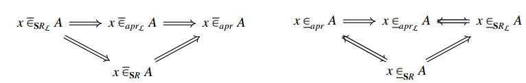
The next example explains the irreversible parts of the implications in these diagrams.

Example 4.3. (1) In Example 4.1 part (1), we have that $A = \{x_1, x_3, x_6\}$, $\overline{apr_\mathcal{L}}(A) = \overline{\mathbf{S}R}(A) = X$ and $\overline{\mathbf{S}R_\mathcal{L}}(A) = A.$ Hence, $x_2, x_4, x_5 \ \overline{\in}_{apr_\mathcal{L}}(A)$ and $x_2, x_4, x_5 \ \overline{\in}_{\mathbf{S}R}(A)$ but $x_2, x_4, x_5\ \overline{\notin}_{\mathbf{S}R_\mathcal{L}}(A).$

(2) In Example 4.1 part (1), we have that $A = \{x_1, x_2\}$, $\overline{apr_\mathcal{L}}(A) = A, \overline{\mathbf{S}R}(A) = \{x_1, x_2, x_5\}$ and $\overline{apr}(A) = X.$ Hence, $x_3, x_4, x_5, x_6 \ \overline{\in}_{apr}(A)$ but $x_3, x_4, x_5, x_6 \ \overline{\notin}_{apr_\mathcal{L}}(A)$ and $x_3, x_4, x_6 \ \overline{\notin}_{\mathbf{S}R}(A).$

(3) In Example 4.1 part (3), we have that $A = \{x_1, x_3, x_6\}$, $\underline{\mathbf{S}R_\mathcal{L}}(A) = A$ and $\underline{\mathbf{S}R}(A) = \{x_6\}$. Hence, $x_1, x_3 \ \underline{\in}_{\mathbf{S}R_\mathcal{L}}(A)$ but, $x_1, x_3 \ \underline{\notin}_{\mathbf{S}R}(A).$

Definition 4.4. Let $P = (X, \mathbf{S}, \mathcal{L})$ be a soft ideal approximation space in which $\mathbf{S} = (F, E)$ is a soft set of $X$ and $A, B\subseteq X.$ Then, the $\mathbf{S}R_\mathcal{L},$ $apr_\mathcal{L}$ and $apr$-soft rough inclusion relations, denoted respectively by $\underset{\rightharpoondown}{\subset}_{\mathbf{S}R_\mathcal{L}}, \overset{\rightharpoonup}{\subset}_{\mathbf{S}R_\mathcal{L}},$ $\underset{\rightharpoondown}{\subset}_{apr_\mathcal{L}}, \overset{\rightharpoonup}{\subset}_{apr_\mathcal{L}}$ and $\underset{\rightharpoondown}{\subset}_{apr}, \overset{\rightharpoonup}{\subset}_{apr},$ are given as follows:

Proposition 4.3. Let $P = (X, \mathbf{S}, \mathcal{L})$ be a soft ideal approximation space in which $\mathbf{S} = (F, E)$ is a soft set of $X$ and $A, B\subseteq X.$ Then, we have the following:

(1) $A\subseteq B \ \Rightarrow \ \ A\underset{\rightharpoondown}{\subset}_{\mathbf{S}R_\mathcal{L}} B,$ $A\underset{\rightharpoondown}{\subset}_{apr_\mathcal{L}} B$ and $A\underset{\rightharpoondown}{\subset}_{apr} B.$

(2) $A\subseteq B \ \Rightarrow \ \ A\overset{\rightharpoonup}{\subset}_{\mathbf{S}R_\mathcal{L}} B,$ $A\overset{\rightharpoonup}{\subset}_{apr_\mathcal{L}} B$ and $A\overset{\rightharpoonup}{\subset}_{apr} B.$

Proof. It follows directly from Definition 4.4, Theorem 2.2 and Propositions 3.2 and 3.4. □

Remark 4.4. The following example explains how the converse of Proposition 4.3 did not hold.

Example 4.4. In Example 4.1, consider that $\mathcal{L} = \{\phi, \{x_2\}, \{x_4\}, \{x_2, x_4\}\}.$ Then, the following holds:

(1) If $A = \{x_1, x_3\}$ and $B = \{x_2, x_4\},$ then $\underline{apr}(A) = \phi, \ \underline{apr_\mathcal{L}}(A) = \{x_1, x_3\}$ and $\underline{apr}(B) = \underline{apr_\mathcal{L}}(B) = \phi.$ Hence, $B\underset{\rightharpoondown}{\subset}_{apr_\mathcal{L}} A$ and $B\underset{\rightharpoondown}{\subset}_{apr} A.$ However, $B\nsubseteq A.$

(2) If $A = \{x_1, x_2\}$ and $B = \{x_1, x_4\},$ then $\overline{apr}(A) = \overline{apr_\mathcal{L}}(A) = X$ and $\overline{apr}(B) = \overline{apr_\mathcal{L}}(B) = X.$ Hence, $A\overset{\rightharpoonup}{\subset}_{apr_\mathcal{L}} B$ and $A\overset{\rightharpoonup}{\subset}_{apr} B.$ However, $A\nsubseteq B.$

Definition 4.5. Let $P = (X, \mathbf{S}, \mathcal{L})$ be a soft ideal approximation space in which $\mathbf{S} = (F, E)$ is a soft set of $X$ and $A, B\subseteq X.$ Then, the $\mathbf{S}R_\mathcal{L}$ and $apr_\mathcal{L}$-soft rough set relations, denoted respectively by ${\eqsim}_{\mathbf{S}R_\mathcal{L}}$, ${\simeq}_{\mathbf{S}R_\mathcal{L}}$ and ${\eqsim}_{apr_\mathcal{L}}$, ${\simeq}_{apr_\mathcal{L}}$ are given as follows:

Remark 4.5. The next example interprets Definition 4.5.

Example 4.5. In Example 4.1, consider that $\mathcal{L} = \{\phi, \{x_3\}\}.$ If $A = \{x_1\}$ and $B = \{x_2\},$ then $\underline{apr_\mathcal{L}}(A) = \underline{\mathbf{S}R_\mathcal{L}}(A) = \underline{apr_\mathcal{L}}(B) = \underline{\mathbf{S}R_\mathcal{L}}(B) = \phi$ and $\overline{apr_\mathcal{L}}(A) = \overline{\mathbf{S}R_\mathcal{L}}(A) = \overline{apr_\mathcal{L}}(B) = \overline{\mathbf{S}R_\mathcal{L}}(B) = X.$ Consequently, $A{\eqsim}_{\mathbf{S}R_\mathcal{L}} B, \; A{\simeq}_{\mathbf{S}R_\mathcal{L}} B, \; A{\approx}_{\mathbf{S}R_\mathcal{L}} B$ and $A{\eqsim}_{apr_\mathcal{L}} B, \; A{\simeq}_{apr_\mathcal{L}} B, \; A{\approx}_{apr_\mathcal{L}} B.$

Proposition 4.4. Let $P = (X, \mathbf{S}, \mathcal{L})$ be a soft ideal approximation space and $A, B, A_1, B_1\subseteq X.$ Then, the following applies:

(1) $A = B\Rightarrow A{\approx}_{\mathbf{S}R_\mathcal{L}} B$ and $A{\approx}_{apr_\mathcal{L}} B.$

(2) $A^c{\eqsim}_{\mathbf{S}R_\mathcal{L}} B^c\Rightarrow A{\eqsim}_{\mathbf{S}R_\mathcal{L}} B$ and $A^c{\simeq}_{\mathbf{S}R_\mathcal{L}} B^c\Rightarrow A{\simeq}_{\mathbf{S}R_\mathcal{L}} B.$

(3) $A{\simeq}_{apr_\mathcal{L}} A_1, \; B{\simeq}_{apr_\mathcal{L}} B_1\Rightarrow (A\cup B){\simeq}_{apr_\mathcal{L}}(A_1\cup B_1).$

(4) $A{\simeq}_{apr_\mathcal{L}} B\Rightarrow A{\simeq}_{apr_\mathcal{L}}(A\cup B){\simeq}_{apr_\mathcal{L}}B$ and $(A\cup B^c){\simeq}_{apr_\mathcal{L}}X.$

(5) $A{\eqsim}_{\mathbf{S}R_\mathcal{L}}\underline{\mathbf{S}R_\mathcal{L}}(A)$, $A{\simeq}_{\mathbf{S}R_\mathcal{L}}\overline{\mathbf{S}R_\mathcal{L}}(A)$ and $A{\eqsim}_{apr_\mathcal{L}}\underline{apr_\mathcal{L}}(A).$

(6) $A\subseteq B, \; B{\eqsim}_{\mathbf{S}R_\mathcal{L}}\phi\Rightarrow A{\eqsim}_{\mathbf{S}R_\mathcal{L}}\phi$ and $A\subseteq B, \; B{\eqsim}_{apr_\mathcal{L}}\phi\Rightarrow A{\eqsim}_{apr_\mathcal{L}}\phi.$

(7) $A\subseteq B, \; B{\simeq}_{\mathbf{S}R_\mathcal{L}}\phi\Rightarrow A{\simeq}_{\mathbf{S}R_\mathcal{L}}\phi$ and $A\subseteq B, \; B{\simeq}_{apr_\mathcal{L}}\phi\Rightarrow A{\simeq}_{apr_\mathcal{L}}\phi.$

(8) $A\subseteq B, \; A{\eqsim}_{\mathbf{S}R_\mathcal{L}}X\Rightarrow B{\eqsim}_{\mathbf{S}R_\mathcal{L}}X$ and $A\subseteq B, \; A{\eqsim}_{apr_\mathcal{L}}X\Rightarrow B{\eqsim}_{apr_\mathcal{L}}X.$

(9) $A\subseteq B, \; A{\simeq}_{\mathbf{S}R_\mathcal{L}}X\Rightarrow B{\simeq}_{\mathbf{S}R_\mathcal{L}}X$ and $A\subseteq B, \; A{\simeq}_{apr_\mathcal{L}}X\Rightarrow B{\simeq}_{apr_\mathcal{L}}X.$

Proof. It follows directly from Definition 4.5 and Propositions 3.2 and 3.4. □

Lemma 4.1. Let $P = (X, \mathbf{S}, \mathcal{L})$ be a soft ideal approximation space and $\mathbf{S} = (F, E)$ be an intersecting complete soft set of $X$. Then, we have

Proof. Usually, $\underline{apr_\mathcal{L}}(A\cap B)\subseteq\underline{apr_\mathcal{L}}(A)\cap\underline{apr_\mathcal{L}}(B).$ Thus, we need to prove the reverse inclusion $\underline{apr_\mathcal{L}}(A\cap B)\supseteq\underline{apr_\mathcal{L}}(A)\cap\underline{apr_\mathcal{L}}(B)$. Let $x\in \underline{apr_\mathcal{L}}(A)\cap\underline{apr_\mathcal{L}}(B).$ Then, there exist $e_1, e_2\in E$ with $x\in F(e_1), F(e_1) \cap A^c\in \mathcal{L}$ and $x\in F(e_2), F(e_2) \cap B^c\in \mathcal{L}.$ By assuming that $\mathbf{S}$ is an intersecting complete soft set, we ensure that there is an $e_3\in E$ with $x\in F(e_3) = F(e_1)\cap F(e_2)$ and $F(e_3) \cap (A\cap B)^c\in \mathcal{L}.$ Hence, we conclude that $x\in\underline{apr_\mathcal{L}}(A\cap B)$. In a similar way, we can deduce that $\underline{\mathbf{S}R_\mathcal{L}}(A\cap B) = \underline{\mathbf{S}R_\mathcal{L}}(A)\cap\underline{\mathbf{S}R_\mathcal{L}}(B).$ □

Proposition 4.5. Let $P = (X, \mathbf{S}, \mathcal{L})$ be a soft ideal approximation space and $\mathbf{S} = (F, E)$ be an intersecting complete soft set of $X$. Then, for $A, B, A_1, B_1\subseteq X,$ we have the following:

(1) $A{\eqsim}_{apr_\mathcal{L}} B\Rightarrow A\cap B^c {\eqsim}_{apr_\mathcal{L}}\phi$ and $A{\eqsim}_{\mathbf{S}R_\mathcal{L}} B\Rightarrow A\cap B^c {\eqsim}_{\mathbf{S}R_\mathcal{L}}\phi.$

(2) $A{\eqsim}_{apr_\mathcal{L}} B\Rightarrow A{\eqsim}_{apr_\mathcal{L}}(A\cap B){\eqsim}_{apr_\mathcal{L}}B$ and $A{\eqsim}_{\mathbf{S}R_\mathcal{L}} B\Rightarrow A{\eqsim}_{\mathbf{S}R_\mathcal{L}}(A\cap B){\eqsim}_{\mathbf{S}R_\mathcal{L}}B.$

(3) $A{\eqsim}_{apr_\mathcal{L}} A_1, \; B{\eqsim}_{apr_\mathcal{L}} B_1\Rightarrow (A\cap B){\eqsim}_{apr_\mathcal{L}}(A_1\cap B_1)$ and $A{\eqsim}_{\mathbf{S}R_\mathcal{L}} A_1, \; B{\eqsim}_{\mathbf{S}R_\mathcal{L}} B_1\Rightarrow (A\cap B){\eqsim}_{\mathbf{S}R_\mathcal{L}}(A_1\cap B_1).$

Proof. It follows directly from Definition 4.5 and Lemma 4.1. □

Proposition 4.6. Let $P = (X, \mathbf{S}, \mathcal{L})$ be a soft ideal approximation space and $\mathbf{S} = (F, E)$ be a soft set of $X$. Then, for all $A\subseteq X$ we have the following:

(1) $\underline{apr_\mathcal{L}}(A) = \bigcap\{B\subseteq X:A{\eqsim}_{apr_\mathcal{L}} B\}$ and $\underline{\mathbf{S}R_\mathcal{L}}(A) = \bigcap\{B\subseteq X:A{\eqsim}_{\mathbf{S}R_\mathcal{L}} B\}.$

(2) $\overline{apr_\mathcal{L}}(A)\supseteq\bigcup\{B\subseteq X:A{\simeq}_{apr_\mathcal{L}} B\}$ and $\overline{\mathbf{S}R_\mathcal{L}}(A) = \bigcup\{B\subseteq X:A{\simeq}_{\mathbf{S}R_\mathcal{L}} B\}.$

Proof. (1) Let $x\in \underline{apr_\mathcal{L}}(A).$ If $A{\eqsim}_{apr_\mathcal{L}} B,$ then $\underline{apr_\mathcal{L}}(A) = \underline{apr_\mathcal{L}}(B).$ But $\underline{apr_\mathcal{L}}(B)\subseteq B$ for any $B\subseteq X.$ It follows that $x\in \underline{apr_\mathcal{L}}(A) = \underline{apr_\mathcal{L}}(B)\subseteq B.$ Hence, $x\in \cap\{B\subseteq X:A{\eqsim}_{apr_\mathcal{L}} B\},$ so $\underline{apr_\mathcal{L}}(A)\subseteq\cap\{B\subseteq X:A{\eqsim}_{apr_\mathcal{L}} B\}.$ Now, we deduce that the reverse inclusion also holds. Let $x\in\cap\{B\subseteq X:A{\eqsim}_{apr_\mathcal{L}} B\}.$ Then, by Proposition 4.4, we have that $A{\eqsim}_{apr_\mathcal{L}}\underline{apr_\mathcal{L}}(A),$ and it follows that $x\in \underline{apr_\mathcal{L}}(A).$ Therefore, $\cap\{B\subseteq X:A{\eqsim}_{apr_\mathcal{L}} B\}\subseteq\underline{apr_\mathcal{L}}(A).$ Consequently, we conclude that $\underline{apr_\mathcal{L}}(A) = \cap\{B\subseteq X:A{\eqsim}_{apr_\mathcal{L}} B\}.$ Similarly, we can deduce that $\underline{\mathbf{S}R_\mathcal{L}}(A) = \bigcap\{B\subseteq X:A{\eqsim}_{\mathbf{S}R_\mathcal{L}} B\}.$

(2) Let $x\in\cup\{B\subseteq X:A{\simeq}_{apr_\mathcal{L}} B\}.$ Then, there exists some $B\subseteq X$ with $x\in B$ and $A{\simeq}_{apr_\mathcal{L}} B.$ But $B \subseteq \overline{apr_\mathcal{L}}(B)$ from Proposition 3.2; thus, $x\in B\subseteq\overline{apr_\mathcal{L}}(B) = \overline{apr_\mathcal{L}}(A).$ Hence, we conclude that $\overline{apr_\mathcal{L}}(A)\supseteq\bigcup\{B\subseteq X:A{\simeq}_{apr_\mathcal{L}} B\}$, as required. Similarly, we can prove that $\overline{\mathbf{S}R_\mathcal{L}}(A)\supseteq\bigcup\{B\subseteq X:A{\simeq}_{\mathbf{S}R_\mathcal{L}} B\}.$ Also, we can deduce that the reverse inclusion $\bigcup\{B\subseteq X:A{\simeq}_{\mathbf{S}R_\mathcal{L}} B\}\supseteq \overline{\mathbf{S}R_\mathcal{L}}(A)$ holds. Let $x\notin\cup\{B\subseteq X:A{\simeq}_{\mathbf{S}R_\mathcal{L}} B\}.$ Then, $x\notin B$ for any $B\subseteq X$ with $A{\simeq}_{\mathbf{S}R_\mathcal{L}} B.$ Thus, by Proposition 4.4, we have that $A{\simeq}_{\mathbf{S}R_\mathcal{L}}\overline{\mathbf{S}R_\mathcal{L}}(A),$ and it follows that $x\notin \overline{\mathbf{S}R_\mathcal{L}}(A).$ Consequently, we conclude that $\overline{\mathbf{S}R_\mathcal{L}}(A) = \cup\{B\subseteq X:A{\simeq}_{\mathbf{S}R_\mathcal{L}} B\}.$ □

Remark 4.6. The following example explains Proposition 4.6.

Example 4.6. In Example 4.1, consider that $\mathcal{L} = \{\phi, \{x_2\}, \{x_4\}, \{x_2, x_4\}\}.$ For $A = \{x_3, x_5\}\subseteq X,$ we have that $\underline{apr_\mathcal{L}}(A) = \underline{\mathbf{S}R_\mathcal{L}}(A) = \{x_3\},$ and $\overline{apr_\mathcal{L}}(A) = \{x_1, x_2, x_3, x_5\}$ with $\overline{\mathbf{S}R_\mathcal{L}}(A) = \{x_2, x_3, x_4, x_5\}.$ Then, one can see that $\underline{apr_\mathcal{L}}(A) = \underline{\mathbf{S}R_\mathcal{L}}(A) = \bigcap\{B\subseteq X:A{\eqsim}_{apr_\mathcal{L}} B\} = \{x_3\}$ and $\overline{\mathbf{S}R_\mathcal{L}}(A) = \bigcup\{B\subseteq X:A{\simeq}_{\mathbf{S}R_\mathcal{L}} B\} = \{x_2, x_3, x_4, x_5\}.$ Also, $\bigcup\{B\subseteq X:A{\simeq}_{apr_\mathcal{L}} B\} = \{x_2, x_3, x_5\}\varsubsetneqq\overline{apr_\mathcal{L}}(A)$ and $\bigcup\{B\subseteq X:A{\simeq}_{apr_\mathcal{L}} B\} = \{x_2, x_3, x_5\}\varsubsetneqq\overline{apr_\mathcal{L}}(A).$

5.   Two approaches for soft rough set approximations based on ideals

In this section, a new generalization derived as based on two ideals of the best method that has been proposed in Definition 3.5, called soft bi-ideal rough set approximations, is presented. This generalization is analyzed by using two distinct methods. Their properties are investigated, and the relationships between these methods are studied.

Definition 5.1. The quadruple $(X, \mathbf{S}, \mathcal{L}_1, \mathcal{L}_2)$ is called a soft bi-ideal approximation space, $\mathbf{S}$ is a soft set defined on $X$, $\mathcal{L}_1, \mathcal{L}_2$ are two ideals on $X$, and $(X, \mathbf{S}, < \mathcal{L}_1, \mathcal{L}_2 > )$ is called a soft ideal approximation space related to $(X, \mathbf{S}, \mathcal{L}_1, \mathcal{L}_2)$. For any subset $A$ of $X$, the lower approximation and the upper approximation, i.e., $(\mathbf{S}R)_{* < \mathcal{L}_1, \mathcal{L}_2 > }(A)$ and $(\mathbf{S}R)_{ < \mathcal{L}_1, \mathcal{L}_2 > }^*(A),$ are defined respectively, as follows:

Remark 5.1. The lower approximation and the upper approximation given in Definition 5.1 are consistent with the approximations given in Definition 3.4 if $\mathcal{L}_1 = \mathcal{L}_2.$ Also, the confirmed properties of the soft approximations in Definition 5.1 are those given in Proposition 3.3.

Definition 5.2. Let $(X, \mathbf{S}, \mathcal{L}_1, \mathcal{L}_2)$ be a soft bi-ideal approximation space. For any subset $A$ of $X$, the soft lower approximation and the soft upper approximation, $\underline{\mathbf{S}R}_{ < \mathcal{L}_1, \mathcal{L}_2 > }(A)$ and $\overline{\mathbf{S}R}_{ < \mathcal{L}_1, \mathcal{L}_2 > }(A),$ are defined respectively, as follows:

Remark 5.2. The lower approximation and the upper approximation given in Definition 5.2 are consistent with the approximations given in Definition 3.5 if $\mathcal{L}_1 = \mathcal{L}_2.$ Also, the confirmed properties of the soft approximations in Definition 5.2 are those given in Proposition 3.4.

Definition 5.3. Let $(X, \mathbf{S}, \mathcal{L}_1, \mathcal{L}_2)$ be a soft bi-ideal approximation space. For any subset $A$ of $X$, the soft lower approximation and the soft upper approximation, $\underline{\mathbf{S}R}_{\mathcal{L}_1, \mathcal{L}_2}(A)$ and $\overline{\mathbf{S}R}_{\mathcal{L}_1, \mathcal{L}_2}(A),$ are defined respectively, as follows:

where $\underline{\mathbf{S}R_{\mathcal{L}_1}}(A)$ and $\overline{\mathbf{S}R_{\mathcal{L}_2}}(A)$ are the lower approximation and the upper approximation of $A$ as related to $\mathcal{L}_i,$ $i\in\{1, 2\}$ as in Definition 3.5.

Remark 5.3. The lower approximation and the upper approximation given in Definition 5.3 are consistent with the approximations given in Definition 3.5 if $\mathcal{L}_1 = \mathcal{L}_2.$ Also, it should be noted that the operators $\underline{\mathbf{S}R}_{\mathcal{L}_1, \mathcal{L}_2}(A)$ and $\overline{\mathbf{S}R}_{\mathcal{L}_1, \mathcal{L}_2}(A)$ satisfy the conditions of the properties given in Proposition 3.4.

Definition 5.4. Let $(X, \mathbf{S}, \mathcal{L}_1, \mathcal{L}_2)$ be a soft bi-ideal approximation space and $A\subseteq X$. Then, the soft boundary regions $Bnd_{{ < \mathcal{L}_1, \mathcal{L}_2 > }}(A)$ and $Bnd_{{\mathcal{L}_1, \mathcal{L}_2}}(A)$ and the soft accuracy measures $Acc_{{ < \mathcal{L}_1, \mathcal{L}_2 > }}(A)$ and $Acc_{{\mathcal{L}_1, \mathcal{L}_2}}(A)$ are defined respectively, as follows:

Theorem 5.1. Let $(X, \mathbf{S}, \mathcal{L}_1, \mathcal{L}_2)$ be a soft bi-ideal approximation space and $A\subseteq X$. Then, the following holds:

(1) $\overline{\mathbf{S}R}_{ < \mathcal{L}_1, \mathcal{L}_2 > }(A)\subseteq\overline{\mathbf{S}R}_{\mathcal{L}_1, \mathcal{L}_2}(A).$

(2) $\underline{\mathbf{S}R}_{\mathcal{L}_1, \mathcal{L}_2}(A)\subseteq\underline{\mathbf{S}R}_{ < \mathcal{L}_1, \mathcal{L}_2 > }(A).$

(3) $Bnd_{{ < \mathcal{L}_1, \mathcal{L}_2 > }}(A)\subseteq Bnd_{{\mathcal{L}_1, \mathcal{L}_2}}(A)$.

(4) $Acc_{{\mathcal{L}_1, \mathcal{L}_2}}(A)\subseteq Acc_{{ < \mathcal{L}_1, \mathcal{L}_2 > }}(A)$.

Proof. (1) Let $x\in\overline{\mathbf{S}R}_{ < \mathcal{L}_1, \mathcal{L}_2 > }(A).$ Then, $x\in A$ or $x\in (\mathbf{S}R)_{ < \mathcal{L}_1, \mathcal{L}_2 > }^*(A).$ So, $x\in A$ or $\forall e\in E:x\in F(e),$ and we get that $F(e) \cap A\notin < \mathcal{L}_1, \mathcal{L}_2 > .$ First choice, if $x\in A,$ then $x\in \overline{\mathbf{S}R_{\mathcal{L}_1}}(A)$ and $x\in \overline{\mathbf{S}R_{\mathcal{L}_2}}(A).$ Thus, $x\in\overline{\mathbf{S}R}_{\mathcal{L}_1, \mathcal{L}_2}(A).$ Second choice, if $\forall e\in E:x\in F(e),$ we have that $F(e) \cap A\notin < \mathcal{L}_1, \mathcal{L}_2 > ;$ then, $F(e) \cap A\notin \mathcal{L}_1$ and $F(e) \cap A\notin \mathcal{L}_2$ $\forall e\in E:x\in F(e),$ and thus $x\notin (\mathbf{S}R_{\mathcal{L}_1})_*(A^c)$ and $x\notin (\mathbf{S}R_{\mathcal{L}_2})_*(A^c).$ That means that $x\in (\mathbf{S}R_{\mathcal{L}_1})^*(A)$ and $x\in (\mathbf{S}R_{\mathcal{L}_2})^*(A)$ by Definition 3.4. Thus, $x\in\overline{\mathbf{S}R_{\mathcal{L}_1}}(A)\cap\overline{\mathbf{S}R_{\mathcal{L}_2}}(A).$ This means that $x\in \overline{\mathbf{S}R}_{\mathcal{L}_1, \mathcal{L}_2}(A).$ Hence, $\overline{\mathbf{S}R}_{ < \mathcal{L}_1, \mathcal{L}_2 > }(A)\subseteq \overline{\mathbf{S}R}_{\mathcal{L}_1, \mathcal{L}_2}(A).$

(2) Let $x\in \underline{\mathbf{S}R}_{\mathcal{L}_1, \mathcal{L}_2}(A).$ Then, $x\in\underline{\mathbf{S}R_{\mathcal{L}_1}}(A)$ or $x\in\underline{\mathbf{S}R_{\mathcal{L}_2}}(A).$ Therefore, for some $e\in E:x\in F(e),$ we have that $F(e) \cap A^c\in \mathcal{L}_1$ or $F(e) \cap A^c\in \mathcal{L}_2.$ Since $\mathcal{L}_1, \mathcal{L}_2 \subseteq < \mathcal{L}_1, \mathcal{L}_2 > ,$ then for some $e\in E:x\in F(e)$ we have that $F(e) \cap A^c\in < \mathcal{L}_1, \mathcal{L}_2 > .$ Thus, $x\in \underline{\mathbf{S}R}_{ < \mathcal{L}_1, \mathcal{L}_2 > }(A).$ Hence, $\underline{\mathbf{S}R}_{\mathcal{L}_1, \mathcal{L}_2}(A)\subseteq\underline{\mathbf{S}R}_{ < \mathcal{L}_1, \mathcal{L}_2 > }(A).$

(3), (4) It is immediately obtained by applying parts (1) and (2). □

Proposition 5.1. Let $(X, \mathbf{S}, \mathcal{L}_1, \mathcal{L}_2)$ be a soft bi-ideal approximation space and $A\subseteq X$. Then, the following holds:

(1) $\overline{\mathbf{S}R}_{ < \mathcal{L}_1, \mathcal{L}_2 > }(A)\subseteq\overline{\mathbf{S}R}_{\mathcal{L}_1, \mathcal{L}_2}(A)\subseteq \overline{\mathbf{S}R_{\mathcal{L}_i}}(A)$ $\forall i\in\{1, 2\}.$

(2) $\underline{\mathbf{S}R_{\mathcal{L}_i}}(A)\subseteq\underline{\mathbf{S}R}_{\mathcal{L}_1, \mathcal{L}_2}(A)\subseteq\underline{\mathbf{S}R}_{ < \mathcal{L}_1, \mathcal{L}_2 > }(A)$ $\forall i\in\{1, 2\}.$

(3) $Bnd_{ < \mathcal{L}_1, \mathcal{L}_2 > }(A)\subseteq Bnd_{\mathcal{L}_1, \mathcal{L}_2}(A)\subseteq Bnd_{\mathbf{S}R_{\mathcal{L}_i}}(A)$ $\forall i\in\{1, 2\}.$

(4) $Acc_{\mathbf{S}R_{\mathcal{L}_i}}(A)\subseteq Acc_{{\mathcal{L}_1, \mathcal{L}_2}}(A)\subseteq Acc_{ < \mathcal{L}_1, \mathcal{L}_2 > }(A)$ $\forall i\in\{1, 2\}.$

Proof. It directly follows from Definition 5.3 and Theorem 5.1. □

Remark 5.4. From Theorem 5.1, we deduce that the boundary region defined by Definition 5.2 is smaller than that boundary region computed by applying Definition 5.3. Consequently, the accuracy value computed based on Definition 5.2 is higher than the accuracy value computed based on Definition 5.3. In the next section, we introduce two medical applications to clarify the advantages of using these recent methods to make a decision.

6.   Medical applications in decision-making problems

In this section, we show the good performance of the aforementioned approaches as compared to their counterpart approaches that exist in literature ^[28,29] by providing two practical applications.

Example 6.1. Medical application: Decision-making for influenza problem:

The aim of this example is to illustrate the advantage of the approximations defined in Definitions 3.2 and 3.5 as the best tools to detect the critical symptoms of influenza infections. The information in Table 5 was adopted from ^[31,32]. In this example, let $(F, E)$ describe the symptoms of patients suspected of having influenza that any hospital would consider before making a decision. The most common symptoms (set of attributes) of influenza are as follows: Fever, respiratory issues, nasal discharge, cough, headache, lethargy and sore throat. It was taken from six patients under medical examination. So, the set of objects is $X = \{x_1, x_2, x_3, x_4, x_5, x_6\},$ and the set of decision attributes is $E = \{e_1, e_2, e_3, e_4, e_5, e_6, e_7\},$ such that

Consider the mapping $F: E\longrightarrow P(X).$ From Table 5, we can deduce that

Therefore, $F(e_1)$ indicates that patients have a fever, and the functional value is the set $\{p_1, p_3, p_4, p_5, p_6\}$. Thus, $(F, E)$ could be described as a set of approximations, as explained in Table 5.

Consider that $\mathcal{L} = \{\phi, \{x_1\}, \{x_2\}, \{x_3\}, \{x_1, x_2\}, \{x_1, x_3\}, \{x_2, x_3\}, \{x_1, x_2, x_3\}\}.$ A comparison between the introduced methods and the previous methods is shown in Tables 6 and 7. For example, take a set of patients $A = \{x_3, x_4, x_5\};$ then, the soft boundary region ($Bnd_{\mathbf{S}R_\mathcal{L}}(A)$) and soft accuracy measure ($Acc_{\mathbf{S}R_\mathcal{L}}(A)$) by Definition 3.5 are $\phi$ and $1,$ respectively. Alternatively, $Bnd_{apr}(A)$ and $Acc{apr}(A)$ are $\{x_1, x_2, x_5, x_6\}$ and $1/3,$ respectively. Also, $Bnd_{\mathbf{S}R}(A)$ and $Acc_{\mathbf{S}R}(A)$ are $\{x_5, x_6\}$ and $1/2,$ respectively, $Bnd_{apr_\mathcal{L}}(A)$ and $Acc_{apr_\mathcal{L}}(A)$ are $\{x_1, x_2, x_5, x_6\}$ and $1/3,$ respectively. If we take another set such that $A = \{x_2, x_4, x_5, x_6\},$ then $Bnd_{\mathbf{S}R_\mathcal{L}}(A)$ and $Acc_{\mathbf{S}R_\mathcal{L}}(A)$) are $\phi$ and $1,$ respectively. Alternatively, $Bnd_{apr}(A)$ and $Acc{apr}(A)$ are $\{x_1, x_3, x_5, x_6\}$ and $1/3,$ respectively. Also, $Bnd_{\mathbf{S}R}(A)$ and $Acc_{\mathbf{S}R}(A)$ are $\{x_3, x_5, x_6\}$ and $2/5,$ respectively and $Bnd_{apr_\mathcal{L}}(A)$ and $Acc_{apr_\mathcal{L}}(A)$ are $\{x_1\}$ and $5/6,$ respectively. According to the above discussion, Definition 3.5 gives us a smaller boundary region and a higher accuracy value than the ones computed using Definition 3.2 and the methods in ^[28,29]. Additionally, it is clear that the proposed approach in Definition 3.2 and its counterpart introduced in ^[29] are different in general. Hence, a decision made according to the calculations of our current technique in Definition 3.5 is more accurate.

Example 6.2. Medical application: Decision-making for a heart attack problem:

The Cardiology Department in Al-Azhar University ^[33], in this example, saved the data showed in Table 8. We used these data and applied the techniques described in Definitions 5.2 and 5.3 to obtain the best decision for heart attacks. Table 8 represents the set of objects (patients) as

and the set of decision parameters (set of symptoms) is $E = \{e_1, e_2, e_3, e_4, e_5\},$ meaning that

The decision of a heart attacks is confirmed by "Decision" as explained in Table 8.

From Table 8, we can deduce that

Consequently, anyone can present two ideals to illustrate that the approximations given in Definition 5.2 are superior to those ones given in Definition 5.3 by extending tables similar to Tables 6 and 7, and by comparing the resultant accuracy.

For example, let $\mathcal{L}_1 = \{\phi, \{x_2\}\}$ and $\mathcal{L}_2 = \{\phi, \{x_3\}, \{x_5\}, \{x_3, x_5\}\}$ be two ideals on $X$. Therefore, we have that $< \mathcal{L}_1, \mathcal{L}_2 > = \{\phi, \{x_2\}, \{x_3\}, \{x_5\}, \{x_2, x_3\}, \{x_2, x_5\}, \{x_3, x_5\}, \{x_2, x_3, x_5\}\}.$

From Table 8, the patients $\{x_6, x_7\}$ were surely diagnosed with heart attacks. Thus, we respectively computed the soft lower, soft upper, soft boundary and soft accuracy measure of $A$ to be given as follows:

(1) The approach in Definition 5.3 yields $\phi,$ $X,$ $X$ and $0.$ This means that the patients $x_6$ and $x_7$ did not experienced heart attacks, which is a contradiction to the "yes" values in Table 8. So, we could not determine whether a patient suffered a heart attack.

(2) The approach in Definition 5.2 yields $\{x_6, x_7\},$ $X,$ $\{x_1, x_2, x_4, x_4, x_5\}$ and $2/7.$ This means that the patients $\{x_6, x_7\}$ surely experienced a heart attack according to the techniques of Definition 5.2 which is consistent with Table 8. As a result, we were able to determine whether a patient suffered a heart attack. Additionally, the soft boundary region decreased and the soft accuracy measure was higher.

At the end, it should be noted that the use of the soft rough technique utilizing ideals as detailed in our new proposal in Definition 5.2 also refines the primary evaluation results of an expert group and thus allows us to select the optimal object in a more reliable manner. Specifically, the soft lower approximation can be used to add the optimal objects that have possibly been neglected by some experts in the primary evaluation, while the soft upper approximation can be used to remove the objects that have been improperly selected as the optimal objects by some experts in the primary evaluation. Therefore, considering that the subjective aspect of decision making is considered and described by using the evaluation soft set in our best method, as based the two ideals in Definition 5.2, the use of soft rough sets could, to some extent, automatically reduce the errors caused by the subjective nature of the evaluation given by an expert group in some decision-making problems.

7.   Conclusions

This paper is a modification and could be a generalization of the roughness of soft sets. Two new approximations called soft ideal rough approximations, which generalize the old soft approximations ^[28,29], have been proposed. It is proved that the two proposed approaches satisfy the conditions of the main properties established in Pawlak's model. Moreover, comparisons among these approaches and previous ones ^[28,29] have been discussed. Moreover, we proved that our second approach defined in Definition 3.5, is the best one since it produces smaller boundary regions and greater accuracy values than the corresponding boundary regions and accuracy values obtained via our first method in Definition 3.2 and those introduced in ^[28,29]. Furthermore, two new soft approximation spaces based on two ideals, called soft bi-ideal approximation spaces, have been introduced in Definitions 5.2 and 5.3. The properties and results of these soft bi-ideal rough sets have been presented. Also, the comparisons between these methods have been investigated. These methods can be extended by using $n$-ideals. The importance of the introduced soft approximations is that they are dependent on the concept of "ideal" which effectively minimizes the ambiguity raised in real-life problems and results in better decisions. Therefore, two medical applications have been offered to highlight the effect of incorporating ideals into the current approaches. We demonstrated in the first proposed application that our strategies reduce border regions and increase the accuracy measure of the sets more than the approaches shown in ^[28,29]. In the second medical application, we proved that the approximations explained in Definition 5.2 yield a smaller boundary and a higher accuracy than those obtained by applying Definition 5.3, and this was achieved by comparing the resultant boundary and accuracy results. In the two medical applications, our techniques handled the imperfect data for symptoms, which automatically made patient diagnosis simple and accurate. As a result, medical personnel can make more accurate decisions about patient diagnosis. In future work, we will introduce the notion of fuzzy soft ideal rough approximation and conduct further research in this direction.

Use of AI tools declaration

The authors declare they have not used Artificial Intelligence (AI) tools in the creation of this article.

Acknowledgments

The authors extend their appreciation to the Deputyship for Research and Innovation, Ministry of Education in Saudi Arabia for funding this research work through the project number ISP-2024.

Conflict of interest

The authors declare that they have no conflict of interest.