Forest model dynamics analysis and optimal control based on disease and fire interactions

Xiaoxiao Liu; Chunrui Zhang; Xiaoxiao Liu; Chunrui Zhang

doi:10.3934/math.2024154

AIMS Mathematics

2024, Volume 9, Issue 2: 3174-3194. doi: 10.3934/math.2024154

Previous Article Next Article

Research article

Forest model dynamics analysis and optimal control based on disease and fire interactions

Xiaoxiao Liu ¹,
Chunrui Zhang ^{2
,
,}

1.
College of Computer and Control Engineering, Northeast Forestry University, Harbin 150040, China
2.
College of Science, Northeast Forestry University, Harbin 150040, China

Received: 08 November 2023 Revised: 24 December 2023 Accepted: 27 December 2023 Published: 03 January 2024
MSC : 34C23, 35K57

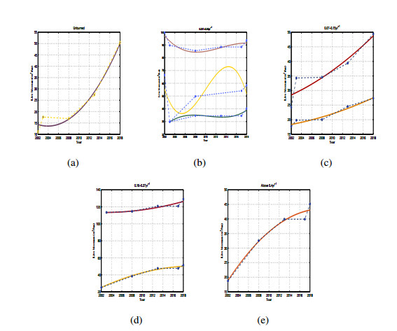
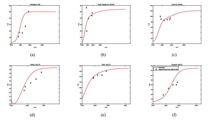
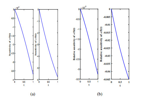
Three models for the propagation of forest disease are revisited to include the effect of forest fires and disease spread. We study the global stability of the forest-disease model in the absence of forest fires and the spread of disease. When forest fires caused by grass cover are considered, we show that the equilibrium points are locally asymptotically stable. If both forest fires and the spread of disease exist in the second model, then Turing instability can occur. In this case, the system exhibits complex dynamic behavior. To determine the effect of fire on the forest disease model, we obtain the optimal control expression of the key parameter fire factor, and carry out sensitivity analysis. Finally, we use forest biomass data of some provinces in China from 2002 to 2018 for numerical simulation, and the results are in agreement with the theoretical analysis.
- Forest-Disease model,
- forest fire,
- stability,
- optimal control,
- sensitivity analysis
Citation: Xiaoxiao Liu, Chunrui Zhang. Forest model dynamics analysis and optimal control based on disease and fire interactions[J]. AIMS Mathematics, 2024, 9(2): 3174-3194. doi: 10.3934/math.2024154

Related Papers:

Abstract

Three models for the propagation of forest disease are revisited to include the effect of forest fires and disease spread. We study the global stability of the forest-disease model in the absence of forest fires and the spread of disease. When forest fires caused by grass cover are considered, we show that the equilibrium points are locally asymptotically stable. If both forest fires and the spread of disease exist in the second model, then Turing instability can occur. In this case, the system exhibits complex dynamic behavior. To determine the effect of fire on the forest disease model, we obtain the optimal control expression of the key parameter fire factor, and carry out sensitivity analysis. Finally, we use forest biomass data of some provinces in China from 2002 to 2018 for numerical simulation, and the results are in agreement with the theoretical analysis.

References

[1]	N. G. Mcdowell, C. D. Allen, A. T. Kristina, Pervasive shifts in forest dynamics in a changing world, Science, 368 (2020), 964–976. http://dx.doi.org/10.1126/science.aaz9463 doi: 10.1126/science.aaz9463
[2]	R. Seidl, D. Thom, M. Kautz, D. Martin-Benito, Forest disturbances under climate change, Nat. Clim. Chang., 7 (2017), 395–402. http://dx.doi.org/10.1038/NCLIMATE3303 doi: 10.1038/NCLIMATE3303
[3]	J. A. Hicke, C. D. Allen, A. R. Desai, Effects of biotic disturbances on forest carbon cycling in the United States and Canada, Glob. Change Biol., 18 (2012), 7–34. http://dx.doi.org/10.1111/j.1365-2486.2011.02543.x doi: 10.1111/j.1365-2486.2011.02543.x
[4]	I. L. Boyd, P. H. Freersmith, C. A. Gilligan, H. C. J. Godfray, The consequence of tree pests and diseases for ecosystem services, Science, 342 (2013), 823–833. http://dx.doi.org/10.1126/science.1235773 doi: 10.1126/science.1235773
[5]	A. J. Tepley, E. Thomann, T. T. Veblen, Influences of fire-vegetation feedbacks and post-fire recovery rates on forest landscape vulnerability to altered fire regimes, J. Ecol., 106 (2018), 1925–1940. http://dx.doi.org/10.1111/1365-2745.12950 doi: 10.1111/1365-2745.12950
[6]	A. C. Staver, S. Archibald, S. A. Levin, The global extent and determinants of savanna and forest as alternative biome states, Science, 334 (2011), 230–232. http://dx.doi.org/10.1126/science.1210465 doi: 10.1126/science.1210465
[7]	S. I. Higgins, W. J. Bond, W. S. W. Trollope, Fire, resprouting and variability: a recipe for grass-tree coexistence in savanna, J. Ecol., 88 (2000), 213–229. http://dx.doi.org/10.1046/j.1365-2745.2000.00435.x doi: 10.1046/j.1365-2745.2000.00435.x
[8]	W. A. Hoffmann, E. L. Geiger, S. G. Gotsch, D. R. Rossatto, L. C. R. Silva, O. L. Lau, Ecological thresholds at the savanna forest boundary: how plant traits, resources and fire govern the distribution of tropical biomes, Ecol. Lett., 15 (2012), 759–768. http://dx.doi.org/10.1111/j.1461-0248.2012.01789.x doi: 10.1111/j.1461-0248.2012.01789.x
[9]	D. W. Peterson, P. B. Reich, K. J. Wrage, J. Franklin, Plant functional group responses to fire frequency and tree canopy cover gradients in oak savannas and woodlands, J. Veg. Sci., 18 (2007), 3–12. http://dx.doi.org/10.1111/j.1654-1103.2007.tb02510.x doi: 10.1111/j.1654-1103.2007.tb02510.x
[10]	R. K. Meentemeyer, N. J. Cunniffe, A. R. Cook, J. A. Joao, R. D. Hunter, D. M. Rizzo, Epidemiological modeling of invasion in heterogeneous landscapes: spread of sudden oak death in California (1990–2030), Ecosphere, 2 (2011), 1–24. http://dx.doi.org/10.1890/ES10-00192.1 doi: 10.1890/ES10-00192.1
[11]	A. Dobson, M. Crawley, Pathogens and the structure of plant communities, Trends Ecol. Evol., 9 (1994), 393–398. http://dx.doi.org/10.1016/0169-5347(94)90062-0 doi: 10.1016/0169-5347(94)90062-0
[12]	R. M. Anderson, R. May, Infectious Diseases of Humans: Dynamics and Control, Oxford: Oxford University Press, 1991. http://dx.doi.org/10.1002/hep.1840150131
[13]	J. J. Burdon, G. A. Chilvers, Host density as a factor in plant disease ecology, Annu. Rev. Phytopathol, 20 (1982), 143–166. http://dx.doi.org/10.1146/annurev.py.20.090182.001043 doi: 10.1146/annurev.py.20.090182.001043
[14]	L. S. Comita, S. A. Queenborough, S. J. Murphy, Testing predictions of the Janzen-Connell hypothesis: a meta-analysis of experimental evidence for distance-and density-dependent seed and seedling survival, J. Ecol., 102 (2014), 845–856. http://dx.doi.org/10.1111/1365-2745.12232 doi: 10.1111/1365-2745.12232
[15]	J. P. Gerlach, P. B. Reich, K. Puettmann, T. Baker, Species, diversity, and density affect tree seedling mortality from Armillaria root rot, Can. J. For. Res., 27 (1997), 1509–1512. http://dx.doi.org/10.1139/x97-098 doi: 10.1139/x97-098
[16]	D. W. Peterson, P. B. Reich, Prescribed fire in oak savanna: fire frequency effects on stand structure and dynamics, Ecol. Appl., 11 (2001), 914–927. http://dx.doi.org/10.1890/1051-0761(2001)011[0914:PFIOSF]2.0.CO;2 doi: 10.1890/1051-0761(2001)011[0914:PFIOSF]2.0.CO;2
[17]	L. E. Frelich, P. B. Reich, D. W. Peterson, Fire in Upper Midwestern Oak Forest Ecosystems: An Oak Forest Restoration and Management Handbook, Portland: Pacific Northwest Research Station, 2015. http://dx.doi.org/10.2737/PNW-GTR-914
[18]	A. F. A. Pellegrini, A. M. Hein, J. Cavender-Bares, R. A. Montgomery, Disease and fire interact to influence transitions between savanna-forest ecosystems over a multi-decadal experiment, Ecol. Lett., 24 (2021), 1007–1017. http://dx.doi.org/10.1111/ele.13719 doi: 10.1111/ele.13719
[19]	P. Magal, Z. Y. Zhang, A system of state-dependent delay differential equation modelling forest growth Ⅱ: Boundedness of solutions, Nonlinear Anal. Real World Appl., 42 (2018), 334–352. http://dx.doi.org/10.1016/j.nonrwa.2018.01.002 doi: 10.1016/j.nonrwa.2018.01.002
[20]	P. Magal, Z. Y. Zhang, A system of state-dependent delay differential equation modeling forest growth Ⅰ: semiflow properties, J. Evol. Equ., 18 (2018), 1853–1888. http://dx.doi.org/10.1007/s00028-018-0464-0 doi: 10.1007/s00028-018-0464-0
[21]	P. Magal, Z. Y. Zhang, Numerical simulations of a population dynamic model describing parasite destruction in a wild type pine forest, Ecol. Complex., 34 (2018), 147–160. http://dx.doi.org/10.1016/j.ecocom.2017.05.001 doi: 10.1016/j.ecocom.2017.05.001
[22]	P. Magal, Z. Y. Zhang, Competition for light in forest population dynamics: from computer simulator to mathematical model, J. Evol. Equ., 419 (2017), 290–304. http://dx.doi.org/10.1016/j.jtbi.2017.02.025 doi: 10.1016/j.jtbi.2017.02.025
[23]	J. P. Tripathi, S. Tyagi, S. Abbas, Global analysis of a delayed density dependent predator-prey model with Crowley-Martin functional response, Commun. Nonlinear Sci. Numer. Simul., 30 (2015), 45–69. http://dx.doi.org/10.1016/j.cnsns.2015.06.008 doi: 10.1016/j.cnsns.2015.06.008
[24]	H. Chen, C. Zhang, Dynamic analysis of a Leslie Gower type predator prey system with the fear effect and ratio-dependent Holling Ⅲ functional response, Nonlinear Anal. Model Control, 27 (2022), 904–926. http://dx.doi.org/10.15388/namc.2022.27.27932 doi: 10.15388/namc.2022.27.27932
[25]	X. M. Rong, M. Fan, H. P. Zhu, Dynamic modeling and optimal control of cystic echinococcosis, Infect. Dis. Poverty, 10 (2021), 38. http://dx.doi.org/10.1186/s40249-021-00807-6 doi: 10.1186/s40249-021-00807-6
[26]	L. H. Zhou, M. Fan, Q. Hou, Z. Jin, X. D. Sun, Transmission dynamics and optimal control of brucellosis in Inner Mongolia of China, Math. Biosci. Eng., 15 (2018), 543–567. http://dx.doi.org/10.3934/mbe.2018025 doi: 10.3934/mbe.2018025
[27]	R. H. Martin, Logarithmic norms and projections applied to linear differential systems, J. Math. Anal. Appl., 45 (1974), 432–454. http://dx.doi.org/10.1016/0022-247X(74)90084-5 doi: 10.1016/0022-247X(74)90084-5
[28]	X. X. Liu, C. R. Zhang, Stability and optimal control of Tree-Insect Model under forest fire disturbance, Mathematics, 10 (2022), 2563. http://dx.doi.org/10.3390/math10152563 doi: 10.3390/math10152563

Reader Comments

Your name:*

Email:*
© 2024 the Author(s), licensee AIMS Press. This is an open access article distributed under the terms of the Creative Commons Attribution License (http://creativecommons.org/licenses/by/4.0)