Selection of artificial neutral networks based on cubic intuitionistic fuzzy Aczel-Alsina aggregation operators

Chunxiao Lu; Zeeshan Ali; Peide Liu; Chunxiao Lu; Zeeshan Ali; Peide Liu

doi:10.3934/math.20241350

AIMS Mathematics

2024, Volume 9, Issue 10: 27797-27833. doi: 10.3934/math.20241350

Previous Article Next Article

Research article

Selection of artificial neutral networks based on cubic intuitionistic fuzzy Aczel-Alsina aggregation operators

1.
School of Tourism, Shandong Women's University, Shandong, Jinan, 250300, China
2.
Department of Information Management, National Yunlin University of Science and Technology, 123 University Road, Section 3, Douliou, Yunlin 64002, Taiwan
3.
Shandong Key Laboratory of New Smart Media, Jinan Shandong 250014, China

Received: 07 August 2024 Revised: 07 September 2024 Accepted: 14 September 2024 Published: 26 September 2024
MSC : 03B52, 03E72, 03E73, 28E10, 94D05

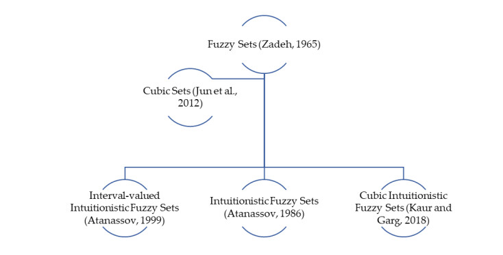
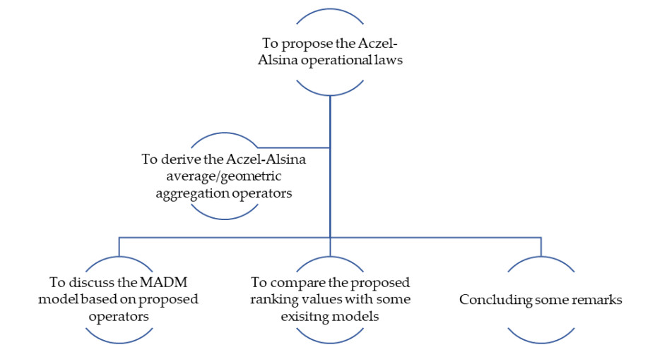
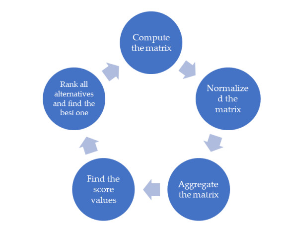
Artificial neural networks (ANNs) are the collection of computational techniques or models encouraged by the shape and purpose of natural or organic neural networks. Furthermore, a cubic intuitionistic fuzzy (CIF) set is the modified or extended form of a Fuzzy set (FS). Our goal was to address or compute the model of Aczel-Alsina operational laws under the consideration of the CIF set as well as Aczel-Alsina t-norm (AATN) and Aczel-Alsina t-conorm (AATCN), where the model of Algebraic norms and Drastic norms were the special parts of the Aczel-Alsina norms. Further, using the above invented operational laws, we aimed to develop the model of Aczel-Alsina average/geometric aggregation operators, called CIF Aczel-Alsina weighted averaging (CIFAAWA), CIF Aczel-Alsina ordered weighted averaging (CIFAAOWA), CIF Aczel-Alsina hybrid averaging (CIFAAHA), CIF Aczel-Alsina weighted geometric (CIFAAWG), CIF Aczel-Alsina ordered weighted geometric (CIFAAOWG), and CIF Aczel-Alsina hybrid geometric (CIFAAHG) operators with some well-known and desirable properties. Moreover, a procedure decision-making technique was presented for finding the best type of artificial neural networks with the help of multi-attribute decision-making (MADM) problems based on CIF aggregation information. Finally, we determined a numerical example for showing the rationality and advantages of the developed method by comparing their ranking values with the ranking values of many prevailing tools.
Citation: Chunxiao Lu, Zeeshan Ali, Peide Liu. Selection of artificial neutral networks based on cubic intuitionistic fuzzy Aczel-Alsina aggregation operators[J]. AIMS Mathematics, 2024, 9(10): 27797-27833. doi: 10.3934/math.20241350

Related Papers:

Abstract

Artificial neural networks (ANNs) are the collection of computational techniques or models encouraged by the shape and purpose of natural or organic neural networks. Furthermore, a cubic intuitionistic fuzzy (CIF) set is the modified or extended form of a Fuzzy set (FS). Our goal was to address or compute the model of Aczel-Alsina operational laws under the consideration of the CIF set as well as Aczel-Alsina t-norm (AATN) and Aczel-Alsina t-conorm (AATCN), where the model of Algebraic norms and Drastic norms were the special parts of the Aczel-Alsina norms. Further, using the above invented operational laws, we aimed to develop the model of Aczel-Alsina average/geometric aggregation operators, called CIF Aczel-Alsina weighted averaging (CIFAAWA), CIF Aczel-Alsina ordered weighted averaging (CIFAAOWA), CIF Aczel-Alsina hybrid averaging (CIFAAHA), CIF Aczel-Alsina weighted geometric (CIFAAWG), CIF Aczel-Alsina ordered weighted geometric (CIFAAOWG), and CIF Aczel-Alsina hybrid geometric (CIFAAHG) operators with some well-known and desirable properties. Moreover, a procedure decision-making technique was presented for finding the best type of artificial neural networks with the help of multi-attribute decision-making (MADM) problems based on CIF aggregation information. Finally, we determined a numerical example for showing the rationality and advantages of the developed method by comparing their ranking values with the ranking values of many prevailing tools.

References

[1]	G. A. Klein, Strategies of decision making, Mil. Rev., 69 (1989), 56–64.
[2]	C. R. Schwenk, Strategic decision making, J. Manag., 21 (1995), 471–493. https://doi.org/10.1016/0149-2063(95)90016-0 doi: 10.1016/0149-2063(95)90016-0
[3]	D. H. Jonassen, designing for decision making, Education Tech. Res. Dev., 60 (2012), 341–359. https://doi.org/10.1007/s11423-011-9230-5 doi: 10.1007/s11423-011-9230-5
[4]	J. Peterson, Decision‐making in the European Union: Towards a framework for analysis, J. Eur. Public Policy, 2 (1995), 69–93. https://doi.org/10.1080/13501769508406975 doi: 10.1080/13501769508406975
[5]	L. A. Zadeh, Fuzzy sets, Inf. Control, 8 (1965), 338–353. https://doi.org/10.1016/S0019-9958(65)90241-X doi: 10.1016/S0019-9958(65)90241-X
[6]	K. Atanassov, Intuitionistic fuzzy sets, Fuzzy Sets Syst., 20 (1986), 87–96. https://doi.org/10.1007/978-3-7908-1870-3_1 doi: 10.1007/978-3-7908-1870-3_1
[7]	K. T. Atanassov, Interval valued intuitionistic fuzzy sets, In: Intuitionistic fuzzy sets: Theory and applications, Heidelberg: Physica, 1999. https://doi.org/10.1007/978-3-7908-1870-3_2
[8]	Y. B. Jun, C. S. Kim, K. O. Yang, Cubic sets, Ann. Fuzzy Math. Inf., 4 (2012), 83–98.
[9]	L. A. Zadeh, Outline of a new approach to the analysis of complex systems and decision processes, IEEE Trans. Syst. Man Cybern., SMC-3 (1973), 28–44. https://doi.org/10.1109/TSMC.1973.5408575
[10]	I. B. Turksen, Interval valued fuzzy sets based on normal forms, Fuzzy Sets Syst., 20 (1986), 191–210. https://doi.org/10.1016/0165-0114(86)90077-1 doi: 10.1016/0165-0114(86)90077-1
[11]	G. Kaur, H. Garg, Multi-attribute decision-making based on Bonferroni mean operators under cubic intuitionistic fuzzy set environment, Entropy, 20 (2018), 65. https://doi.org/10.3390/e20010065 doi: 10.3390/e20010065
[12]	A. Mardani, M. Nilashi, E. K. Zavadskas, S. R. Awang, H. Zare, N. M. Jamal, Decision making methods based on fuzzy aggregation operators: Three decades review from 1986 to 2017, Int. J. Inf. Tech. Decis. Making, 17 (2018), 391–466. https://doi.org/10.1142/S021962201830001X doi: 10.1142/S021962201830001X
[13]	J. M. Merigó, M. Casanovas, Fuzzy Generalized Hybrid Aggregation Operators and its Application in Fuzzy Decision Making, Int. J. Fuzzy Syst., 12 (2010), 11–22. https://doi.org/10.1142/S021962201830001 doi: 10.1142/S021962201830001
[14]	Z. Xu, Intuitionistic fuzzy aggregation operators, IEEE Trans. Fuzzy Syst., 15 (2007), 1179–1187. https://doi.org/10.1109/TFUZZ.2006.890678 doi: 10.1109/TFUZZ.2006.890678
[15]	X. Yu, Z. Xu, Prioritized intuitionistic fuzzy aggregation operators, Inf. Fusion, 14 (2013), 108–116. https://doi.org/10.1016/j.inffus.2012.01.011 doi: 10.1016/j.inffus.2012.01.011
[16]	Z. Xu, R. R. Yager, Some geometric aggregation operators based on intuitionistic fuzzy sets, Int. J. General Syst., 35 (2006), 417–433. https://doi.org/10.1080/03081070600574353 doi: 10.1080/03081070600574353
[17]	H. Garg, Z. Ali, T. Mahmood, M. R. Ali, A. Alburaikan, Schweizer-Sklar prioritized aggregation operators for intuitionistic fuzzy information and their application in multi-attribute decision-making, Alex. Eng. J., 67 (2023), 229–240. https://doi.org/10.1016/j.aej.2022.12.049 doi: 10.1016/j.aej.2022.12.049
[18]	W. Wang, X. Liu, Y. Qin, Interval-valued intuitionistic fuzzy aggregation operators, J. Syst. Eng. Electron., 23 (2012), 574–580. https://doi.org/10.1109/JSEE.2012.00071 doi: 10.1109/JSEE.2012.00071
[19]	T. Senapati, R. Mesiar, V. Simic, A. Iampan, R. Chinram, R. Ali, Analysis of interval-valued intuitionistic fuzzy aczel–alsina geometric aggregation operators and their application to multiple attribute decision-making, Axioms, 11 (2022), 258. https://doi.org/10.3390/axioms11060258 doi: 10.3390/axioms11060258
[20]	X. Shi, Z. Ali, T. Mahmood, P. Liu, Power Aggregation Operators of Interval-Valued Atanassov-Intuitionistic Fuzzy Sets Based on Aczel–Alsina t-Norm and t-Conorm and Their Applications in Decision Making, Int. J. Comput. Intell. Syst., 16 (2023), 43. https://doi.org/10.1007/s44196-023-00208-7 doi: 10.1007/s44196-023-00208-7
[21]	G. Wei, X. Wang, Some geometric aggregation operators based on interval-valued intuitionistic fuzzy sets and their application to group decision making, 2007 International Conference on Computational Intelligence and Security (CIS 2007), 2007,495–499. https://doi.org/10.1109/CIS.2007.84
[22]	Z. Xu, J. Chen, On geometric aggregation over interval-valued intuitionistic fuzzy information. Fourth International Conference on Fuzzy Systems and Knowledge Discovery (FSKD 2007), 2007,466–471. https://doi.org/10.1109/FSKD.2007.427
[23]	A. Fahmi, F. Amin, S. Abdullah, A. Ali, Cubic fuzzy Einstein aggregation operators and its application to decision-making, Int. J. Syst. Sci., 49 (2018), 2385–2397. https://doi.org/10.1080/00207721.2018.1503356 doi: 10.1080/00207721.2018.1503356
[24]	A. Khan, A. U. Jan, F. Amin, A. Zeb, Multiple attribute decision-making based on cubical fuzzy aggregation operators, Granul. Comput., 7 (2022), 393–410. https://doi.org/10.1007/s41066-021-00273-3 doi: 10.1007/s41066-021-00273-3
[25]	G. Kaur, H. Garg, Cubic intuitionistic fuzzy aggregation operators, Int. J. Uncertainty Quantif., 8 (2018), 405–427. https://doi.org/10.1615/Int.J.UncertaintyQuantification.2018020471 doi: 10.1615/Int.J.UncertaintyQuantification.2018020471
[26]	G. Kaur, H. Garg, Generalized cubic intuitionistic fuzzy aggregation operators using t-norm operations and their applications to group decision-making process, Arabian J. Sci. Eng., 44 (2019), 2775–2794. https://doi.org/10.1007/s13369-018-3532-4 doi: 10.1007/s13369-018-3532-4
[27]	E. P. Klement, P. Mesiar, Triangular norms, Tatra Mt. Math. Publ., 13 (1997), 169–193.
[28]	J. Aczél, C. Alsina, Characterizations of some classes of quasilinear functions with applications to triangular norms and to synthesizing judgements, Aeq. Math., 25 (1992), 313–315. https://doi.org/10.1007/BF02189626 doi: 10.1007/BF02189626
[29]	T. Senapati, G. Chen, R. R. Yager, Aczel–Alsina aggregation operators and their application to intuitionistic fuzzy multiple attribute decision making, Int. J. Intell. Syst., 37 (2022), 1529–1551. https://doi.org/10.1002/int.22684 doi: 10.1002/int.22684
[30]	T. Senapati, G. Chen, R. Mesiar, R. R. Yager, Novel Aczel–Alsina operations‐based interval‐valued intuitionistic fuzzy aggregation operators and their applications in multiple attribute decision‐making process, Int. J. Intell. Syst., 37 (2022), 5059–5081. https://doi.org/10.1002/int.22751 doi: 10.1002/int.22751
[31]	T. Senapati, G. Chen, R. Mesiar, R. R. Yager, A. Saha, Novel Aczel–Alsina operations-based hesitant fuzzy aggregation operators and their applications in cyclone disaster assessment, Int. J. Gen. Syst., 51 (2022), 511–546. https://doi.org/10.1080/03081079.2022.2036140 doi: 10.1080/03081079.2022.2036140
[32]	T. Mahmood, Z. Ali, S. Baupradist, R. Chinram, Complex intuitionistic fuzzy Aczel-Alsina aggregation operators and their application in multi-attribute decision-making, Symmetry, 14 (2022), 2255. https://doi.org/10.3390/sym14112255 doi: 10.3390/sym14112255
[33]	T. Senapati, G. Chen, R. Mesiar, R. R. Yager, Intuitionistic fuzzy geometric aggregation operators in the framework of Aczel-Alsina triangular norms and their application to multiple attribute decision making, Expert. Syst. Appl., 212 (2023), 118832. https://doi.org/10.1016/j.eswa.2022.118832 doi: 10.1016/j.eswa.2022.118832
[34]	J. Ahmmad, T. Mahmood, N. Mehmood, K. Urawong, R. Chinram, Intuitionistic Fuzzy Rough Aczel-Alsina Average Aggregation Operators and Their Applications in Medical Diagnoses, Symmetry, 14 (2022), 2537. https://doi.org/10.3390/sym14122537 doi: 10.3390/sym14122537
[35]	M. Sarfraz, K. Ullah, M. Akram, D. Pamucar, D. Božanić, Prioritized aggregation operators for intuitionistic fuzzy information based on Aczel–Alsina T-norm and T-conorm and their applications in group decision-making, Symmetry, 14 (2022), 2655. https://doi.org/10.3390/sym14122655 doi: 10.3390/sym14122655
[36]	T. Mahmood, Z. Ali, Multi-attribute decision-making methods based on Aczel–Alsina power aggregation operators for managing complex intuitionistic fuzzy sets, Comp. Appl. Math., 42 (2023), 87. https://doi.org/10.1007/s40314-023-02204-1 doi: 10.1007/s40314-023-02204-1
[37]	A. Hussain, H. Wang, H. Garg, K. Ullah, An Approach to Multi-attribute Decision Making Based on Intuitionistic Fuzzy Rough Aczel-Alsina Aggregation Operators, J. King Saud Univ.-Sci., 35 (2023), 102760. https://doi.org/10.1016/j.jksus.2023.102760 doi: 10.1016/j.jksus.2023.102760
[38]	M. R. Seikh, U. Mandal, Intuitionistic fuzzy Dombi aggregation operators and their application to multiple attribute decision-making, Granul. Comput., 6 (2021), 473–488. https://doi.org/10.1007/s41066-019-00209-y doi: 10.1007/s41066-019-00209-y
[39]	M. R. Seikh, U. Mandal, q-Rung orthopair fuzzy Archimedean aggregation operators: application in the site selection for software operating units, Symmetry, 15 (2023), 1680. https://doi.org/10.3390/sym15091680 doi: 10.3390/sym15091680
[40]	M. R. Seikh, U. Mandal, Q-rung orthopair fuzzy Frank aggregation operators and its application in multiple attribute decision-making with unknown attribute weights, Granul. Comput., 7 (2022), 709–730. https://doi.org/10.1007/s41066-021-00290-2 doi: 10.1007/s41066-021-00290-2
[41]	M. R. Seikh, U. Mandal, Multiple attribute group decision making based on quasirung orthopair fuzzy sets: Application to electric vehicle charging station site selection problem, Eng. Appl. Artif. Intell, 115 (2022), 105299. https://doi.org/10.1016/j.engappai.2022.105299 doi: 10.1016/j.engappai.2022.105299
[42]	M. R. Seikh, U. Mandal, Multiple attribute decision-making based on 3, 4-quasirung fuzzy sets, Granul. Comput., 7 (2022), 965–978. https://doi.org/10.1007/s41066-021-00308-9 doi: 10.1007/s41066-021-00308-9
[43]	H. M. A. Farid, S. Dabic-Miletic, M. Riaz, V. Simic, D. Pamucar, Prioritization of sustainable approaches for smart waste management of automotive fuel cells of road freight vehicles using the q-rung orthopair fuzzy CRITIC-EDAS method, Inf. Sci., 661 (2024), 120162. https://doi.org/10.1016/j.ins.2024.120162 doi: 10.1016/j.ins.2024.120162
[44]	M. Riaz, M. R. Hashmi, Linear Diophantine fuzzy set and its applications towards multi-attribute decision-making problems, J. Intell. Fuzzy Syst., 37 (2022), 5417–5439. https://doi.org/10.3233/JIFS-190550 doi: 10.3233/JIFS-190550
[45]	M. Riaz, R. Kausar, T. Jameel, D. Pamucar, Cubic picture fuzzy topological data analysis with integrating blockchain and the metaverse for uncertain supply chain management, Eng. Appl. Artif. Intell., 131 (2024), 107827. https://doi.org/10.1016/j.engappai.2023.107827 doi: 10.1016/j.engappai.2023.107827
[46]	A. Razzaq, M. Riaz, Picture fuzzy soft-max Einstein interactive weighted aggregation operators with applications, Comput. Appl. Math., 43 (2024), 90–104. https://doi.org/10.1007/s40314-024-02609-6 doi: 10.1007/s40314-024-02609-6

Reader Comments

Your name:*

Email:*
© 2024 the Author(s), licensee AIMS Press. This is an open access article distributed under the terms of the Creative Commons Attribution License (http://creativecommons.org/licenses/by/4.0)