Obesity treatment applying effective fuzzy soft multiset-based decision-making process

Hanan H. Sakr; Hanan H. Sakr

doi:10.3934/math.20241302

AIMS Mathematics

2024, Volume 9, Issue 10: 26765-26798. doi: 10.3934/math.20241302

Previous Article Next Article

Research article Special Issues

Obesity treatment applying effective fuzzy soft multiset-based decision-making process

Hanan H. Sakr ^{1,2
,
,}

1.
Department of Management Information Systems, College of Business Administration in Hawtat Bani Tamim, Prince Sattam Bin Abdulaziz University, Saudi Arabia
2.
Department of Mathematics, Faculty of Education, Ain Shams University, Cairo 11341, Egypt

Received: 23 July 2024 Revised: 28 August 2024 Accepted: 04 September 2024 Published: 14 September 2024
MSC : 03E72, 03E05, 92C50

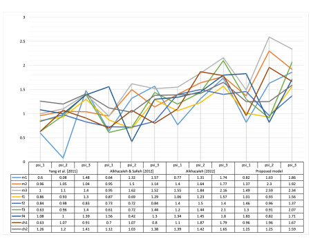
Nowadays, obesity is recognized as a worldwide epidemic that has become a major cause of death and comorbidities. Recommending appropriate treatment is critical in the global health environment. For obesity treatment to be effective, the person must be able to follow a specific diet that meets his needs so that he can follow it for a long time or forever to maintain fitness. This research aims to determine the best diet among the trusted diets for every person based on his needs and circumstances. This occurs when applying a decision-making technique based on the effective fuzzy soft multiset concept. For this purpose, the definition of the effective fuzzy soft multiset as well as its types, operations, and properties are introduced. Furthermore, a decision-making method is proposed based on the effective fuzzy soft multiset environment. Using matrices operations, one can easily apply the decision-making process based on this new extension of sets to choose the optimal diet for everyone. Finally, an extensive comparative analysis of the previous methods is undertaken and also summarized in a chart to attract focus on the benefits of the suggested algorithm and to demonstrate how they differ from the current one.
- decision-making,
- effective set,
- fuzzy set,
- multiset,
- soft set
Citation: Hanan H. Sakr. Obesity treatment applying effective fuzzy soft multiset-based decision-making process[J]. AIMS Mathematics, 2024, 9(10): 26765-26798. doi: 10.3934/math.20241302

Related Papers:

Abstract

Nowadays, obesity is recognized as a worldwide epidemic that has become a major cause of death and comorbidities. Recommending appropriate treatment is critical in the global health environment. For obesity treatment to be effective, the person must be able to follow a specific diet that meets his needs so that he can follow it for a long time or forever to maintain fitness. This research aims to determine the best diet among the trusted diets for every person based on his needs and circumstances. This occurs when applying a decision-making technique based on the effective fuzzy soft multiset concept. For this purpose, the definition of the effective fuzzy soft multiset as well as its types, operations, and properties are introduced. Furthermore, a decision-making method is proposed based on the effective fuzzy soft multiset environment. Using matrices operations, one can easily apply the decision-making process based on this new extension of sets to choose the optimal diet for everyone. Finally, an extensive comparative analysis of the previous methods is undertaken and also summarized in a chart to attract focus on the benefits of the suggested algorithm and to demonstrate how they differ from the current one.

References

[1]	J. Ahmed, M. A. Alam, A. Mobin, S. Tarannum, A soft computing approach for obesity assessment, In: Proceedings of the 5th International Conference on Reliability, Infocom Technologies and Optimization (ICRITO), IEEE, 2016. https://doi.org/10.1109/ICRITO.2016.7784946
[2]	M. A. Al Hashemi, Luqaimat Diet, Egypt: Akhbar Al-Youm Press House, 2009.
[3]	S. Alkhazaleh, Effective fuzzy soft set theory and its applications, Appl. Comput. Intell. Soft Comput., 2020, 6469745. https://doi.org/10.1155/2022/6469745 doi: 10.1155/2022/6469745
[4]	S. Alkhazaleh, A. R. Salleh, Fuzzy soft multiset theory, Abst. Appl. Anal., 2012, 350603. https://doi.org/10.1155/2012/350603 doi: 10.1155/2012/350603
[5]	S. Alkhazaleh, A. R. Salleh, N. Hassan, Soft multisets theory, Appl. Math. Sci., 5 (2011), 3561–3573.
[6]	M. N. P. Alperin, G. Berzosa, A fuzzy logic approach to measure overweight, working papers, 2011.
[7]	J. Axe, Keto Diet: Your 30-Day Plan To Lose Weight, Balance Hormones, Boost Brain Health, And Reverse Disease, United Kingdom: Orion Spring, 2019.
[8]	T. M. Basu, N. K. Mahapatra, S. K. Mondal, Different types of matrices in fuzzy soft set theory and their application in decision-making problems, Int. J. Managm. IT Eng., 2 (2012), 389–398.
[9]	N. Ça$\breve{g}$man, S. Engino$\breve{g}$lu, Soft matrix theory and its decision-making, Comput. Math. Appl., 59 (2010), 3308–3314. https://doi.org/10.1016/j.camwa.2010.03.015 doi: 10.1016/j.camwa.2010.03.015
[10]	A. A. El-Atik, R. Abu-Gdairi, A. A. Nasef, S. Jafari, M. Badr, Fuzzy soft sets and decision making in ideal nutrition, Symmetry, 15 (2023), 1523. https://doi.org/10.3390/sym15081523 doi: 10.3390/sym15081523
[11]	S. I. Farhad, A. M. Chowdhury, E. Adnan, J. N. Moni, R. R. Arif, A. H. Sakib, et al., Fuzzy logic-based weight balancing, Adv. Intell. Sys. Comput., 764 (2019).
[12]	N. Faried, M. S. S. Ali, H. H. Sakr, Fuzzy soft inner product spaces, Appl. Math. Inf. Sci., 14 (2020), 709–720. http://dx.doi.org/10.18576/amis/140419 doi: 10.18576/amis/140419
[13]	N. Faried, M. S. S. Ali, H. H. Sakr, Fuzzy soft Hilbert spaces, J. Math. Comp. Sci., 22 (2021), 142–157. http://dx.doi.org/10.22436/jmcs.022.02.06 doi: 10.22436/jmcs.022.02.06
[14]	N. Faried, M. S. S. Ali, H. H. Sakr, On fuzzy soft linear operators in fuzzy soft Hilbert spaces, Abst. Appl. Anal., 2020, 5804957. https://doi.org/10.1155/2020/5804957 doi: 10.1155/2020/5804957
[15]	N. Faried, M. S. S. Ali, H. H. Sakr, Fuzzy soft symmetric operators. Annl. Fuzzy Math. Inform., 19 (2020), 275–280. https://doi.org/10.30948/afmi.2020.19.3.275 doi: 10.30948/afmi.2020.19.3.275
[16]	N. Faried, M. S. S. Ali, H. H. Sakr, Fuzzy soft hermitian operators, Adv. Math. Sci. J., 9 (2020), 73–82. https://doi.org/10.37418/amsj.9.1.7 doi: 10.37418/amsj.9.1.7
[17]	N. Faried, M. S. S. Ali, H. H. Sakr, A note on FS isometry operators, Math. Sci. Lett., 10 (2021), 1–3. http://dx.doi.org/10.18576/msl/100101 doi: 10.18576/msl/100101
[18]	N. Faried, M. S. S. Ali, H. H. Sakr, On FS normal operators, Math. Sci. Lett., 10 (2021), 41–46. http://dx.doi.org/10.18576/msl/100202 doi: 10.18576/msl/100202
[19]	N. Faried, M. S. S. Ali, H. H. Sakr, A theoretical approach on unitary operators in fuzzy soft settings, Math. Sci. Lett., 11 (2022), 45–49. http://dx.doi.org/10.18576/msl/110104 doi: 10.18576/msl/110104
[20]	O. Hofmekler, D. Holtzberg, The Warrior Diet: Switch on Your Biological Powerhouse For High Energy, Explosive Strength, and a Leaner, Harder, New York: Dragon Door Publications, 2001.
[21]	A. Kumar, M. Kaur, A new algorithm for solving network flow problems with fuzzy arc lengths, Turk. J. Fuzzy Syst., 2 (2011), 1–13.
[22]	V. Longo, The Longevity Diet, New York: Penguin Books Ltd, 2018.
[23]	P. K. Maji, R. Biswas, A. R. Roy, Soft set theory, Comput. Math. Appl., 45 (2003), 555–562. https://doi.org/10.1016/S0898-1221(03)00016-6 doi: 10.1016/S0898-1221(03)00016-6
[24]	P. K. Maji, A. R. Roy, R. Biswas, An application of soft sets in a decision-making problem, Comput. Math. Appl., 44 (2002), 1077–1083. https://doi.org/10.1016/S0898-1221(02)00216-X doi: 10.1016/S0898-1221(02)00216-X
[25]	D. Molodtsov, Soft set theory-First results, Comput. Math. Appl., 37 (1999), 19–31. https://doi.org/10.1016/S0898-1221(99)00056-5 doi: 10.1016/S0898-1221(99)00056-5
[26]	M. Mosley, M. Spencer, The Fast Diet: Revised and Updated: Lose Weight, Stay healthy, Live longer, New York: Short Books Ltd, 2014.
[27]	M. Saqlain, M. Saeed, From ambiguity to clarity: unraveling the power of similarity measures in multi-polar interval-valued intuitionistic fuzzy soft sets, Decis. Making Adv., 2 (2024), 48–59. https://doi.org/10.31181/dma21202421 doi: 10.31181/dma21202421
[28]	G. Tang, J. Long, X. Gu, F. Chiclana, P. Liu, F. Wang, Interval type-2 fuzzy programming method for risky multicriteria decision-making with heterogeneous relationship, Inform. Sci., 584 (2022), 184–211. https://doi.org/10.1016/j.ins.2021.10.044 doi: 10.1016/j.ins.2021.10.044
[29]	G. Tang, Y. Yang, X. Gu, F. Chiclana, P. Liu, F. Wang, A new integrated multi-attribute decision-making approach for mobile medical app evaluation under q-rung orthopair fuzzy environment, Expert Syst. Appl., 200 (2022), 117034. https://doi.org/10.1016/j.eswa.2022.117034 doi: 10.1016/j.eswa.2022.117034
[30]	G. Tang, X. Gu, F. Chiclana, P. Liu, K. Yin, A multi-objective q-rung orthopair fuzzy programming approach to heterogeneous group decision making, Inform. Sci., 645 (2023), 119343. https://doi.org/10.1016/j.ins.2023.119343 doi: 10.1016/j.ins.2023.119343
[31]	G. Tang, X. Zhang, B. Zhu, H. Seiti, F. Chiclana, P. Liu, A mathematical programming method based on prospect theory for online physician selection under an R-set environment, Inform. Fusion, 93 (2023), 441–468. https://doi.org/10.1016/j.inffus.2023.01.006 doi: 10.1016/j.inffus.2023.01.006
[32]	Y. Yang, C. Ji, Fuzzy soft matrices and their applications, Art. Intell. Comput. Intell., 2011,618–627.
[33]	L. A. Zadeh, Fuzzy sets, Inf. Control, 8 (1965), 338–353. https://doi.org/10.1016/S0019-9958(65)90241-X doi: 10.1016/S0019-9958(65)90241-X

Reader Comments

Your name:*

Email:*
© 2024 the Author(s), licensee AIMS Press. This is an open access article distributed under the terms of the Creative Commons Attribution License (http://creativecommons.org/licenses/by/4.0)