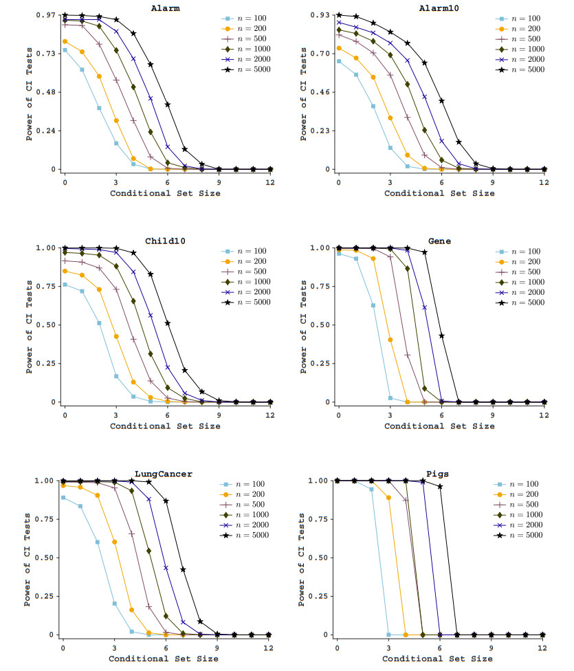
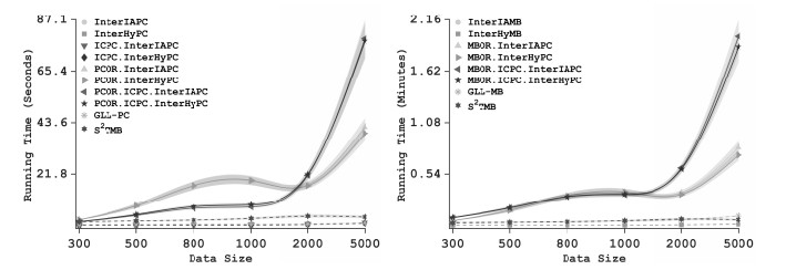
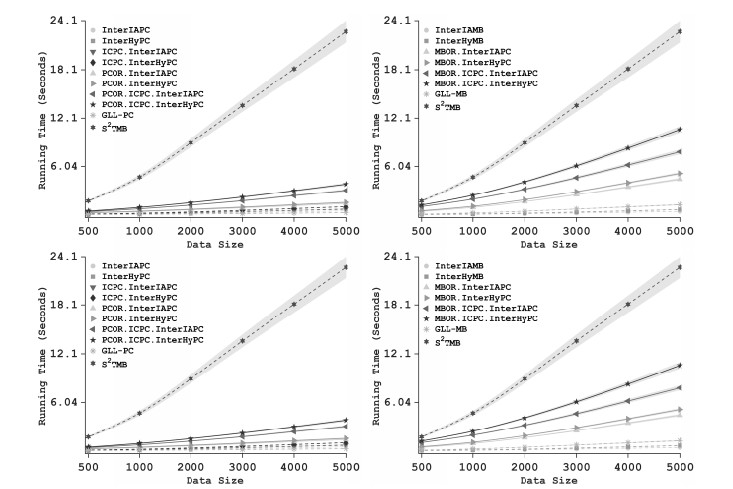
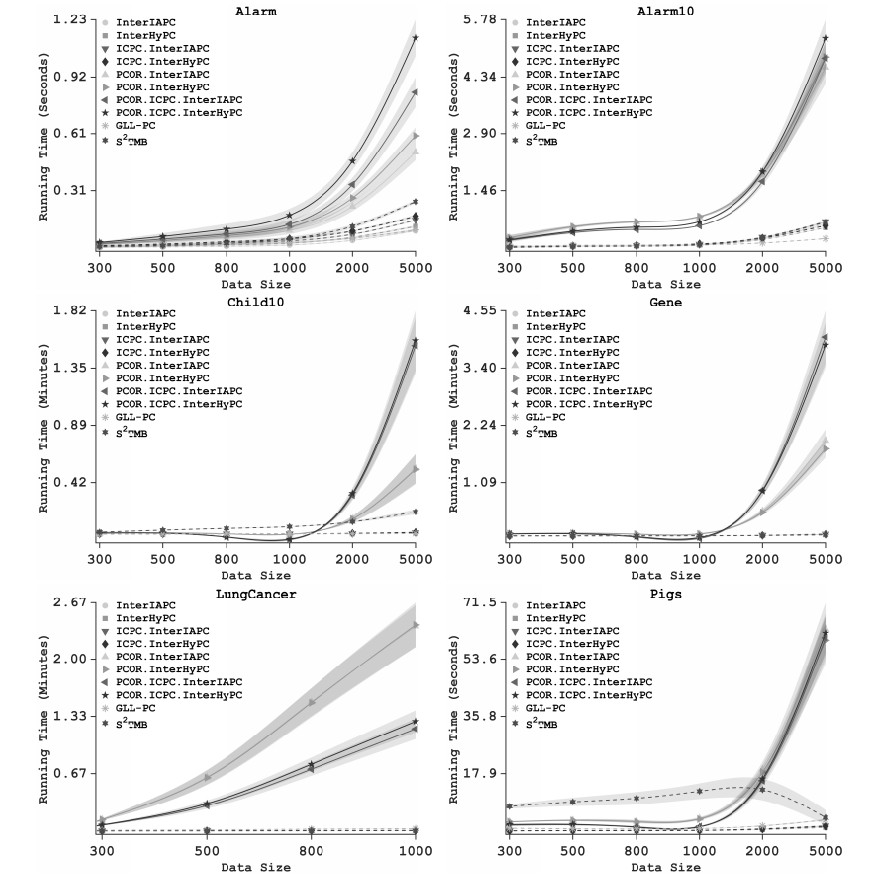
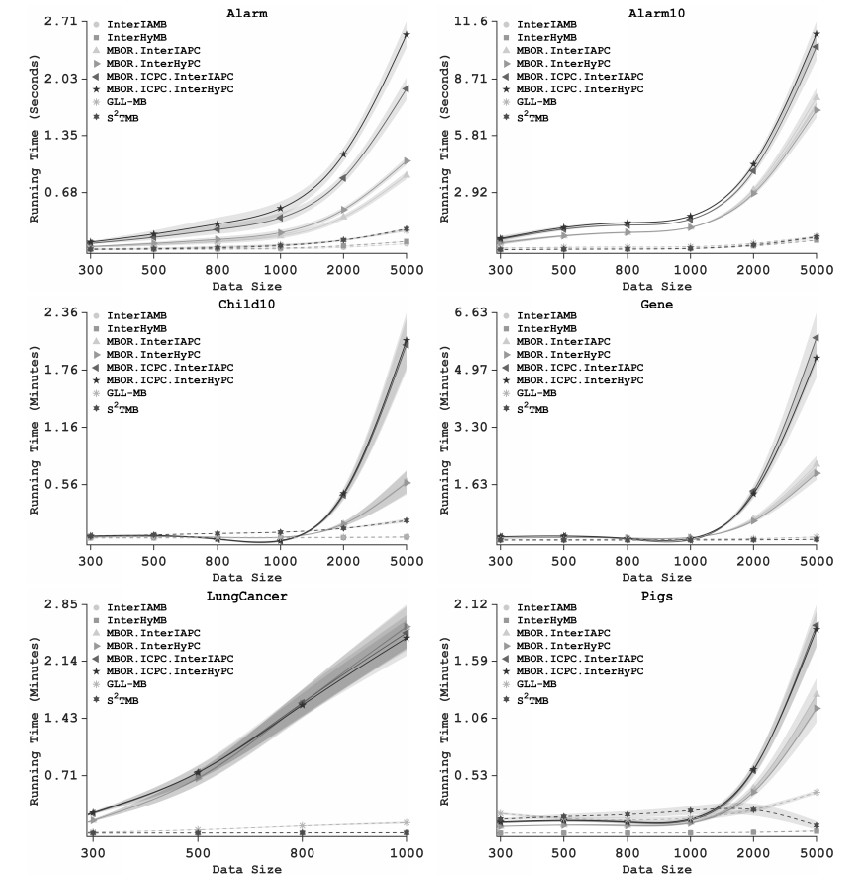
Local discovery in Bayesian networks by information-connecting

Jianying Rong; Xuqing Liu; Jianying Rong; Xuqing Liu

doi:10.3934/math.20241108

AIMS Mathematics

2024, Volume 9, Issue 8: 22743-22793. doi: 10.3934/math.20241108

Previous Article Next Article

Research article

Local discovery in Bayesian networks by information-connecting

Jianying Rong ^{1
,
,},
Xuqing Liu ^{2
,
,}

1.
Department of Quality Education, Jiangsu Vocational College of Electronics and Information, Huai'an 223003, China
2.
Faculty of Mathematics and Physics, Huaiyin Institute of Technology, Huai'an 223003, China

Received: 19 December 2023 Revised: 17 June 2024 Accepted: 01 July 2024 Published: 23 July 2024
MSC : 68T20, 94A15

Local discovery plays an important role in Bayesian networks (BNs), mainly addressing PC (parents and children) discovery and MB (Markov boundary) discovery. In this paper, we considered the problem of large local discovery. First, we focused on an assumption about conditional independence (CI) tests: We explained why it was unreasonable to assume all CI tests were reliable in large local discovery, studied how the power and reliability of CI tests changed with the data size and the number of degrees of freedom, and then modified the assumption about CI tests in a more reasonable way. Second, we concentrated on improving local discovery algorithms: We posed the problem of premature termination of the forward search, analyze why it arose frequently in large local discovery when implementing the existing local discovery algorithms, put forward an idea of preventing the premature termination of forward search called information connection (IC), and used IC to build a novel algorithm called ICPC; the theoretical basis of ICPC was detailedly presented. In addition, a more steady incremental algorithm as the subroutine of ICPC was proposed. Third, the way of breaking ties among equal associations was considered and optimized. Finally, we conducted a benchmarking study by means of six synthetic BNs from various domains. The experimental results revealed the applicability and superiority of ICPC in solving the problem of premature termination of the forward search that arose frequently in large local discovery.
- Bayesian network,
- local discovery,
- PC discovery,
- MB discovery,
- information connection
Citation: Jianying Rong, Xuqing Liu. Local discovery in Bayesian networks by information-connecting[J]. AIMS Mathematics, 2024, 9(8): 22743-22793. doi: 10.3934/math.20241108

Related Papers:

Abstract

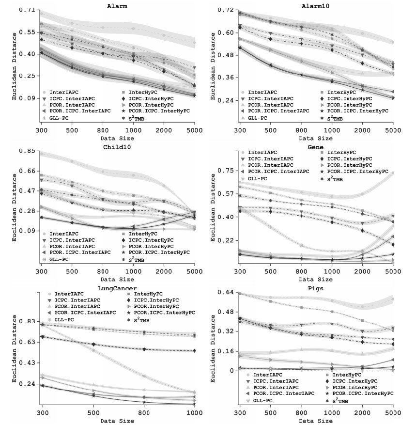
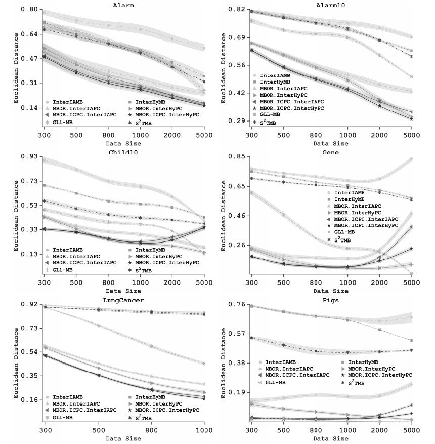
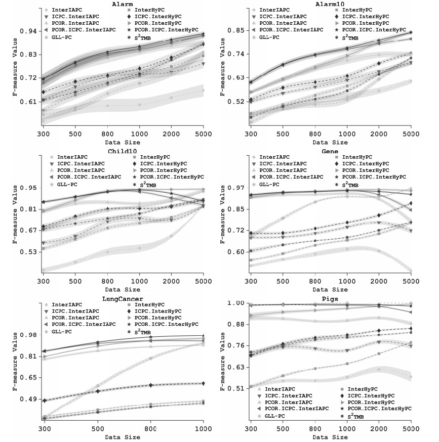
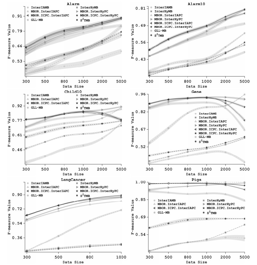
Local discovery plays an important role in Bayesian networks (BNs), mainly addressing PC (parents and children) discovery and MB (Markov boundary) discovery. In this paper, we considered the problem of large local discovery. First, we focused on an assumption about conditional independence (CI) tests: We explained why it was unreasonable to assume all CI tests were reliable in large local discovery, studied how the power and reliability of CI tests changed with the data size and the number of degrees of freedom, and then modified the assumption about CI tests in a more reasonable way. Second, we concentrated on improving local discovery algorithms: We posed the problem of premature termination of the forward search, analyze why it arose frequently in large local discovery when implementing the existing local discovery algorithms, put forward an idea of preventing the premature termination of forward search called information connection (IC), and used IC to build a novel algorithm called ICPC; the theoretical basis of ICPC was detailedly presented. In addition, a more steady incremental algorithm as the subroutine of ICPC was proposed. Third, the way of breaking ties among equal associations was considered and optimized. Finally, we conducted a benchmarking study by means of six synthetic BNs from various domains. The experimental results revealed the applicability and superiority of ICPC in solving the problem of premature termination of the forward search that arose frequently in large local discovery.

References

[1]	J. Pearl, Probabilistic reasoning in intelligent systems: Networks of plausible inference, San Francisco: Morgan Kaufmann, 1988.
[2]	R. E. Neapolitan, Learning bayesian networks, Upper Saddle River: Prentice Hall, 2004.
[3]	R. Daly, Q. Shen, S. Aitken, Learning bayesian networks: Approaches and issues, Knowl. Eng. Rev., 26 (2011), 99–157. https://doi.org/10.1017/S0269888910000251 doi: 10.1017/S0269888910000251
[4]	P. Parviainen, M. Koivisto, Finding optimal bayesian networks using precedence constraints, J. Mach. Learn. Res., 14 (2013), 1387–1415. https://www.jmlr.org/papers/volume14/parviainen13a/parviainen13a.pdf
[5]	L. W. Zhang, H. P. Guo, Introduction to bayesian networks, Beijing: Science Press, 2006.
[6]	N. Friedman, I. Nachman, D. Peér, Learning Bayesian network structure from massive datasets: The "sparse candidate" algorithm, arXiv Preprint, 2013.
[7]	I. Tsamardinos, L. E. Brown, C. F. Aliferis, The max-min hill-climbing Bayesian network structure learning algorithm, Mach. Learn., 65 (2006), 31–78. https://doi.org/10.1007/s10994-006-6889-7
[8]	C. F. Aliferis, A. Statnikov, I. Tsamardinos, S. Mani, X. D. Koutsoukos, Local causal and Markov blanket induction for causal discovery and feature selection for classification part Ⅰ: Algorithms and empirical evaluation, J. Mach. Learn. Res., 11 (2010), 171–234. https://www.jmlr.org/papers/volume11/aliferis10a/aliferis10a.pdf
[9]	C. F. Aliferis, A. Statnikov, I. Tsamardinos, S. Mani, X. D. Koutsoukos, Local causal and Markov blanket induction for causal discovery and feature selection for classification part Ⅱ: Analysis and extensions, J. Mach. Learn. Res., 11 (2010), 235–284. https://www.jmlr.org/papers/volume11/aliferis10b/aliferis10b.pdf
[10]	S. R. de Morais, A. Aussem, A novel Markov boundary based feature subset selection algorithm, Neurocomputing, 73 (2010), 578–584. https://doi.org/10.1016/j.neucom.2009.05.018 doi: 10.1016/j.neucom.2009.05.018
[11]	S. Fu, M. C. Desmarais, Markov blanket based feature selection: A review of past decade, In: Proceedings of the World Congress on Engineering, 2010,321–328.
[12]	F. Schlüter, A survey on independence-based Markov networks learning, Artif. Intell. Rev., 42 (2014), 1069–1093. https://doi.org/10.1007/s10462-012-9346-y doi: 10.1007/s10462-012-9346-y
[13]	J. P. Pellet, A. Elisseeff, Using Markov blankets for causal structure learning, J. Mach. Learn. Res., 9 (2008), 1295–1342. https://www.jmlr.org/papers/volume9/pellet08a/pellet08a.pdf
[14]	A. R. Masegosa, S. Moral, A Bayesian stochastic search method for discovering markov boundaries, Knowl.-Based Syst., 35 (2012), 211–223. https://doi.org/10.1016/j.knosys.2012.04.028 doi: 10.1016/j.knosys.2012.04.028
[15]	I. Tsamardinos, C. F. Aliferis, Towards principled feature selection: Relevancy, filters and wrappers, In: International Workshop on Artificial Intelligence and Statistics, 2003,300–307.
[16]	A. Statnikov, N. I. Lytkin, J. Lemeire, C. F. Aliferis, Algorithms for discovery of multiple Markov boundaries, J. Mach. Learn. Res., 14 (2013), 499–566. https://www.jmlr.org/papers/volume14/statnikov13a/statnikov13a.pdf
[17]	X. Q. Liu, X. S. Liu, Swamping and masking in Markov boundary discovery, Mach. Learn., 104 (2016), 25–54. https://doi.org/10.1007/s10994-016-5545-0 doi: 10.1007/s10994-016-5545-0
[18]	X. Q. Liu, X. S. Liu, Markov blanket and markov boundary of multiple variables, J. Mach. Learn. Res., 19 (2018), 1–50. https://www.jmlr.org/papers/volume19/14-033/14-033.pdf
[19]	N. K. Kitson, A. C. Constantinou, Z. G. Guo, Y. Liu, K. Chobtham, A survey of Bayesian network structure learning, Artif. Intell. Rev., 56 (2023), 8721–8814. https://doi.org/10.1007/s10462-022-10351-w doi: 10.1007/s10462-022-10351-w
[20]	J. Lemeire, Learning causal models of multivariate systems and the value of it for the performance modeling of computer programs, ASP/VUBPRESS/UPA, 2007.
[21]	J. Lemeire, S. Meganck, F. Cartella, T. T. Liu, Conservative independence-based causal structure learning in absence of adjacency faithfulness, Int. J. Approx. Reason., 53 (2012), 1305–1325. https://doi.org/10.1016/j.ijar.2012.06.004 doi: 10.1016/j.ijar.2012.06.004
[22]	F. Bromberg, D. Margaritis, Improving the reliability of causal discovery from small datasets using argumentation, J. Mach. Learn. Res., 10 (2009), 301–340. https://www.jmlr.org/papers/volume10/bromberg09a/bromberg09a.pdf
[23]	J. M. Peña, R. Nilsson, J. Björkegren, J. Tegnér, Towards scalable and data efficient learning of Markov boundaries, Int. J. Approx. Reason., 45 (2007), 211–232. https://doi.org/10.1016/j.ijar.2006.06.008 doi: 10.1016/j.ijar.2006.06.008
[24]	J. Cheng, R. Greiner, J. Kelly, D. Bell, W. R. Liu, Learning Bayesian networks from data: An information-theory based approach, Artif. Intell., 137 (2002), 43–90. https://doi.org/10.1016/S0004-3702(02)00191-1 doi: 10.1016/S0004-3702(02)00191-1
[25]	H. Cramér, Mathematical methods of statistics, New Jersey: Princeton University Press, 1999.
[26]	S. Kullback, Information theory and statistics, New York: Dover Publications, 1997.
[27]	L. M. de Campos, A scoring function for learning Bayesian networks based on mutual information and conditional independence tests, J. Mach. Learn. Res., 7 (2006), 2149–2187. https://www.jmlr.org/papers/volume7/decampos06a/decampos06a.pdf
[28]	W. G. Cochran, Some methods for strengthening the common $\chi^2$ tests, Biometrics, 10 (1954), 417–451. https://doi.org/10.2307/3001616 doi: 10.2307/3001616
[29]	D. N. Lawley, A general method for approximating to the distribution of likelihood ratio criteria, Biometrika, 43 (1956), 295–303. https://doi.org/10.2307/2332908 doi: 10.2307/2332908
[30]	B. S. Hosmane, Improved likelihood ratio tests and pearson chi-square tests for independence in two dimensional contingency tables, Commun. Stat.-Theor. M., 15 (1986), 1875–1888. https://doi.org/10.1080/03610928608829224 doi: 10.1080/03610928608829224
[31]	B. S. Hosmane, Improved likelihood ratio test for multinomial goodness of fit, Commun. Stat.-Theor. M., 16 (1987), 3185–3198. https://doi.org/10.1080/03610928708829566 doi: 10.1080/03610928708829566
[32]	B. S. Hosmane, Smoothing of likelihood ratio statistic for equiprobable multinomial goodness-of-fit, Ann. Inst. Stat. Math., 42 (1990), 133–147. https://doi.org/10.1007/BF00050784 doi: 10.1007/BF00050784
[33]	S. Brin, R. Motwani, C. Silverstein, Beyond market baskets: Generalizing association rules to correlations, Proceedings of the 1997 ACM SIGMOD International Conference on Management of Data, 26 (1997), 265–276. https://doi.org/10.1145/253260.253327 doi: 10.1145/253260.253327
[34]	C. Silverstein, S. Brin, R. Motwani, Beyond market baskets: Generalizing association rules to dependence rules, Data Min. Knowl. Disc., 2 (1998), 39–68. https://doi.org/10.1023/A:1009713703947 doi: 10.1023/A:1009713703947
[35]	S. Yaramakala, Fast Markov blanket discovery, Iowa State University, 2004.
[36]	P. Spirtes, C. Glymour, R. Scheines, Causation, prediction, and search, Cambridge: MIT Press, 2001.
[37]	S. K. Fu, M. Desmarais, Local learning algorithm for Markov blanket discovery, Advances in Artificial Intelligence, 2007, 68–79.
[38]	W. Khan, L. F. Kong, S. M. Noman, B. Brekhna, A novel feature selection method via mining Markov blanket, Appl. Intell., 53 (2023), 8232–8255. https://doi.org/10.1007/s10489-022-03863-z doi: 10.1007/s10489-022-03863-z
[39]	D. Koller, M. Sahami, Toward optimal feature selection, In: Thirteen International Conference in Machine Learning, Stanford InfoLab, 1996,284–292.
[40]	D. Margaritis, S. Thrun, Bayesian network induction via local neighborhoods, Carnegie Mellon University, 1999.
[41]	D. Margaritis, S. Thrun, Bayesian network induction via local neighborhoods, In: Advances in Neural Information Processing Systems, Morgan Kaufmann, 1999,505–511.
[42]	I. Tsamardinos, C. F. Aliferis, A. Statnikov, Algorithms for large scale Markov blanket discovery, In: Proceedings of the Sixteenth International Florida Artificial Intelligence Research Society Conference (FLAIRS), 2003,376–381.
[43]	X. L. Yang, Y. J. Wang, Y. Ou, Y. H. Tong, Three-fast-inter incremental association Markov blanket learning algorithm, Pattern Recogn. Lett., 122 (2019), 73–78. https://doi.org/10.1016/j.patrec.2019.02.002 doi: 10.1016/j.patrec.2019.02.002
[44]	H. R. Liu, Q. R. Shi, Y. B. Cai, N. T. Wang, L.Y. Zhang, D. Y. Liu, Fast shrinking parents-children learning for markov blanket-based feature selection, Int. J. Mach. Learn. Cyber., 15 (2024), 3553–3566. https://doi.org/10.1007/s13042-024-02108-4 doi: 10.1007/s13042-024-02108-4
[45]	K. P. Murphy, Bayes Net Toolbox for matlab, Version: FullBNT-1.0.7, 2007. Available from: https://github.com/bayesnet/bnt
[46]	T. Gao, Q. Ji, Efficient score-based Markov blanket discovery, Int. J. Approx. Reason., 80 (2017), 277–293. https://doi.org/10.1016/j.ijar.2016.09.009 doi: 10.1016/j.ijar.2016.09.009
[47]	T. Niinimäki, P. Parviainen, Local structure disocvery in Bayesian network, arXiv Preprint, 2012.
[48]	T. Silander, P. Myllymäki, A simple approach for finding the globally optimal bayesian network structure, arXiv Preprint, 2012.
[49]	J. Cussens, M. Bartlett, E. M. Jones, N. A. Sheehan, Maximum likelihood pedigree reconstruction using integer linear programming, Genet. Epidemiol., 37 (2013), 69–83. https://doi.org/10.1002/gepi.21686 doi: 10.1002/gepi.21686
[50]	G. Brown, A. Pocock, M. J. Zhao, M. Luján, Conditional likelihood maximisation: A unifying framework for information theoretic feature selection, J. Mach. Learn. Res., 13 (2012), 27–66. https://www.jmlr.org/papers/volume13/brown12a/brown12a.pdf
[51]	K. T. Fang, J. L. Xu, Statistical distributions, Beijing: Science Press, 1987.
[52]	N. L. Johnson, S. Kotz, Distributions in statistics: Continuous univariate distributions-2, Boston: John Wiley & Sons, 1970.
[53]	G. Schwarz, Estimating the dimension of a model, Ann. Stat., 6 (1978), 461–464. https://www.jstor.org/stable/2958889

Reader Comments

Your name:*

Email:*
© 2024 the Author(s), licensee AIMS Press. This is an open access article distributed under the terms of the Creative Commons Attribution License (http://creativecommons.org/licenses/by/4.0)