Incorporating stochastic volatility and long memory into geometric Brownian motion model to forecast performance of Standard and Poor's 500 index

Mohammed Alhagyan; Mansour F. Yassen; Mohammed Alhagyan; Mansour F. Yassen

doi:10.3934/math.2023945

AIMS Mathematics

2023, Volume 8, Issue 8: 18581-18595. doi: 10.3934/math.2023945

Previous Article Next Article

Research article

Incorporating stochastic volatility and long memory into geometric Brownian motion model to forecast performance of Standard and Poor's 500 index

Mohammed Alhagyan ^{1
,
,},
Mansour F. Yassen ^1,2

1.
Mathematics Department, College of Humanities and Science in Al Aflaj, Prince Sattam Bin Abdulaziz University, Saudi Arabia
2.
Department of Mathematics, Faculty of Science, Damietta University, New Damietta 34517 Damietta, Egypt

Received: 25 March 2023 Revised: 18 May 2023 Accepted: 19 May 2023 Published: 01 June 2023
MSC : 62Pxx, 91Gxx

It is known in the financial world that the index price reveals the performance of economic progress and financial stability. Therefore, the future direction of index prices is a priority of investors. This empirical study investigated the effect of incorporating memory and stochastic volatility into geometric Brownian motion (GBM) by forecasting the future index price of S&P 500. To conduct this investigation, a comparison study was implemented between twelve models; six models without memory (GBM) and six models with memory (GFBM) under two different assumptions of volatility; constant, which were computed by three methods, and stochastic volatility, obeying three deterministic functions. The results showed that the best performance model was for GFBM under a stochastic volatility assumption using the identity deterministic function $ \sigma \left({Y}_{t}\right) = {Y}_{t} $, according to the smallest values of mean square error (MSE) and mean average percentage error (MAPE). This revealed the direct positive effect of incorporating memory and stochastic volatility into GBM to forecast index prices, and thus can be applied in a real financial environment. Furthermore, the findings showed invalidity of the models with exponential deterministic function $ \sigma \left({Y}_{t}\right) = {e}^{{Y}_{t}} $ in forecasting index prices according to huge values of MAPE and MSE.
- geometric Brownian motion,
- geometric fractional Brownian motion,
- stochastic volatility,
- long memory,
- S&P 500
Citation: Mohammed Alhagyan, Mansour F. Yassen. Incorporating stochastic volatility and long memory into geometric Brownian motion model to forecast performance of Standard and Poor's 500 index[J]. AIMS Mathematics, 2023, 8(8): 18581-18595. doi: 10.3934/math.2023945

Related Papers:

Abstract

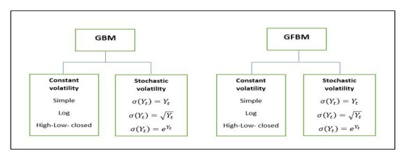
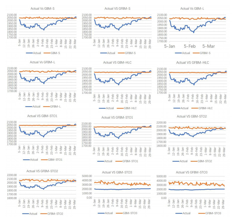
It is known in the financial world that the index price reveals the performance of economic progress and financial stability. Therefore, the future direction of index prices is a priority of investors. This empirical study investigated the effect of incorporating memory and stochastic volatility into geometric Brownian motion (GBM) by forecasting the future index price of S&P 500. To conduct this investigation, a comparison study was implemented between twelve models; six models without memory (GBM) and six models with memory (GFBM) under two different assumptions of volatility; constant, which were computed by three methods, and stochastic volatility, obeying three deterministic functions. The results showed that the best performance model was for GFBM under a stochastic volatility assumption using the identity deterministic function $ \sigma \left({Y}_{t}\right) = {Y}_{t} $, according to the smallest values of mean square error (MSE) and mean average percentage error (MAPE). This revealed the direct positive effect of incorporating memory and stochastic volatility into GBM to forecast index prices, and thus can be applied in a real financial environment. Furthermore, the findings showed invalidity of the models with exponential deterministic function $ \sigma \left({Y}_{t}\right) = {e}^{{Y}_{t}} $ in forecasting index prices according to huge values of MAPE and MSE.

References

[1]	F. Black, M. Scholes, The pricing of options and corporate liabilities, J. Polit. Econ., 81 (1973), 637–654. https://doi.org/10.1086/260062 doi: 10.1086/260062
[2]	S. L. Heston, A closed-form solution for options with stochastic volatility with applications to bond and currency options, Rev. Financ. Stud., 6 (1993), 327–343. https://doi.org/10.1093/rfs/6.2.327 doi: 10.1093/rfs/6.2.327
[3]	J. Hull, A. White, The pricing of options on assets with stochastic volatilities, J. Financ., 42 (1987), 281–300. https://doi.org/10.1111/j.1540-6261.1987.tb02568.x doi: 10.1111/j.1540-6261.1987.tb02568.x
[4]	Y. El-Khatib, A. Hatemi-J, Computations of price sensitivities after a financial market crash, In: Electrical engineering and intelligent systems, New York, NY: Springer, 2013,239–248. http://doi.org/10.1007/978-1-4614-2317-1_20
[5]	Y. El-Khatib, M. A. Hajji, M. Al-Refai, Options pricing in jump diffusion markets during financial crisis, Appl. Math. Inform. Sci., 7 (2013), 2319–2326. http://doi.org/10.12785/amis/070623 doi: 10.12785/amis/070623
[6]	Y. El-Khatib, Q. M. Al-Mdallal, Numerical simulations for the pricing of options in jump diffusion markets, Arab J. Math. Sci., 18 (2012), 199–208. https://doi.org/10.1016/j.ajmsc.2011.10.001 doi: 10.1016/j.ajmsc.2011.10.001
[7]	M. Al hagyan, Modeling financial environments using geometric fractional Brownian motion model with long memory stochastic volatility, PhD. thesis, Universiti Utara Malaysia, 2018.
[8]	S. Lin, X. J. He, Analytically pricing variance and volatility swaps with stochastic volatility, stochastic equilibrium level and regime switching, Expert Syst. Appl., 217 (2023), 119592. https://doi.org/10.1016/j.eswa.2023.119592 doi: 10.1016/j.eswa.2023.119592
[9]	X. J. He, S. Lin, Analytically pricing exchange options with stochastic liquidity and regime switching, J. Futures Markets, 43 (2023), 662–676. https://doi.org/10.1002/fut.22403 doi: 10.1002/fut.22403
[10]	P. Pasricha, X. J. He, Exchange options with stochastic liquidity risk, Expert Syst. Appl., 223 (2023), 119915. https://doi.org/10.1016/j.eswa.2023.119915 doi: 10.1016/j.eswa.2023.119915
[11]	X. J. He, S. Lin, A closed-form pricing formula for European options under a new three-factor stochastic volatility model with regime switching, Japan J. Indust. Appl. Math., 40 (2023), 525–536. https://doi.org/10.1007/s13160-022-00538-7 doi: 10.1007/s13160-022-00538-7
[12]	L. Bachelier, Théorie de la speculation, Annales scientifiques de l'École normale supérieure, 17 (1900), 21–86.
[13]	S. M. Ross, An introduction to mathematical finance: options and other topics, 2 Eds., Cambridge University Press, 2002. https://doi.org/10.1017/CBO9780511800634
[14]	U. F. Wiersema, Brownian motion calculus, John Wiley & Sons, 2008
[15]	Y. Aït‐Sahalia, A. Lo, Nonparametric estimation of state‐price densities implicit in financial asset prices, J. Financ., 53 (1998), 499–547. https://doi.org/10.1111/0022-1082.215228 doi: 10.1111/0022-1082.215228
[16]	M. Alhagyan, The effects of incorporating memory and stochastic volatility into GBM to forecast exchange rates of Euro, Alex. Eng. J., 61 (2022), 9601–9608. https://doi.org/10.1016/j.aej.2022.03.036 doi: 10.1016/j.aej.2022.03.036
[17]	C. Han, Y. Wang, Y. Xu, Nonlinearity and efficiency dynamics of foreign exchange markets: evidence from multifractality and volatility of major exchange rates, Economic Research-Ekonomska Istraživanja, 33 (2020), 731–751. https://doi.org/10.1080/1331677X.2020.1734852 doi: 10.1080/1331677X.2020.1734852
[18]	K. Kim, N. Kim, D. Ju, J. Ri, Efficient hedging currency options in fractional Brownian motion model with jumps, Physica A, 539 (2020), 122868. https://doi.org/10.1016/j.physa.2019.122868 doi: 10.1016/j.physa.2019.122868
[19]	E. Balabana, S. Lu, Color of noise: comparative analysis of sub-periodic variation in empirical Hurst exponent across foreign currency changes and their pairwise differences, preprint.
[20]	I. Z. Rejichi, C. Aloui, Hurst exponent behavior and assessment of the MENA stock markets efficiency, Res. Int. Bus. Financ., 26 (2012), 353–370. https://doi.org/10.1016/j.ribaf.2012.01.005 doi: 10.1016/j.ribaf.2012.01.005
[21]	P. Grau-Carles, Empirical evidence of long-range correlations in stock returns, Physica A, 287 (2000), 396–404. https://doi.org/10.1016/S0378-4371(00)00378-2 doi: 10.1016/S0378-4371(00)00378-2
[22]	W. Willinger, M. Taqqu, V. Teverovsky, Stock market prices and long-range dependence, Finance Stochast., 3 (1999), 1–13. https://doi.org/10.1007/s007800050049 doi: 10.1007/s007800050049
[23]	S. Painter, Numerical method for conditional simulation of Levy random fields, Mathematical Geology, 30 (1998), 163–179. https://doi.org/10.1023/A:1021724513646 doi: 10.1023/A:1021724513646
[24]	Y. S. Mishura, Stochastic calculus for fractional Brownian motion and related processes, Berlin, Heidelberg: Springer, 2008. https://doi.org/10.1007/978-3-540-75873-0
[25]	F. Biagini, Y. Hu, B. Øksendal, T. Zhang, Stochastic calculus for fractional Brownian motion and applications, London: Springer, 2008. https://doi.org/10.1007/978-1-84628-797-8
[26]	J. Stein, Overreactions in the options market, J. Financ., 44 (1989), 1011–1023. https://doi.org/10.1111/j.1540-6261.1989.tb02635.x doi: 10.1111/j.1540-6261.1989.tb02635.x
[27]	G. Bakshi, C. Cao, Z. Chen, Pricing and hedging long-term options, J. Econometrics, 94 (2000), 277–318. https://doi.org/10.1016/S0304-4076(99)00023-8 doi: 10.1016/S0304-4076(99)00023-8
[28]	M. Iseringhausen, The time-varying asymmetry of exchange rate returns: a stochastic volatility–stochastic skewness model, J. Empir. Financ., 58 (2020), 275–292. https://doi.org/10.1016/j.jempfin.2020.06.008 doi: 10.1016/j.jempfin.2020.06.008
[29]	J. Hull, A. White, The pricing of options on assets with stochastic volatilities, J. Financ., 42 (1987), 281–300. https://doi.org/10.1111/j.1540-6261.1987.tb02568.x doi: 10.1111/j.1540-6261.1987.tb02568.x
[30]	A. Chronopoulou, F. G. Viens, Stochastic volatility and option pricing with long-memory in discrete and continuous time, Quant. Financ., 12 (2012), 635–649. https://doi.org/10.1080/14697688.2012.664939 doi: 10.1080/14697688.2012.664939
[31]	E. M. Stein, J. C. Stein, Stock price distributions with stochastic volatility: an analytic approach, Rev. Financ. Stud., 4 (1991), 727–752. https://doi.org/10.1093/rfs/4.4.727 doi: 10.1093/rfs/4.4.727
[32]	P. S. Hagan, D. Kumar, A. S. Lesniewski, D. E. Woodward, Managing smile risk, Wilmott, 1 (2002), 84–108.
[33]	S. L. Heston, A closed-form solution for options with stochastic volatility with applications to bond and currency options, Rev. Financ. Stud., 6 (1993), 327–343. https://doi.org/10.1093/rfs/6.2.327 doi: 10.1093/rfs/6.2.327
[34]	F. Comte, E. Renault, Long memory in continuous‐time stochastic volatility models, Math. Financ., 8 (1998), 291–323. https://doi.org/10.1111/1467-9965.00057 doi: 10.1111/1467-9965.00057
[35]	J. Gatheral, T. Jaisson, M. Rosenbaum, Volatility is rough, Quant. Financ., 18 (2018), 933–949. https://doi.org/10.1080/14697688.2017.1393551 doi: 10.1080/14697688.2017.1393551
[36]	X. Wang, W. Zhang, Parameter estimation for long-memory stochastic volatility at discrete observation, Abstr. Appl. Anal., 2014 (2014), 462982. https://doi.org/10.1155/2014/462982 doi: 10.1155/2014/462982
[37]	M. Alhagyan, F. Al-Duais, Forecasting the performance of Tadawul all share index (TASI) using geometric Brownian motion and geometric fractional Brownian motion, Adv. Appl. Stat., 62 (2020), 55–65. http://doi.org/10.17654/AS062010055 doi: 10.17654/AS062010055
[38]	M. Alhagyan, M. Misiran, Z. Omar, Geometric fractional Brownian motion perturbed by fractional Ornstein-Uhlenbeck process and application on KLCI option pricing, Open Access Library Journal, 3 (2016), e2863. http://doi.org/10.4236/oalib.1102863 doi: 10.4236/oalib.1102863
[39]	M. Alhagyan, M. Misiran, Z. Omar, Discussions on continuous stochastic volatility models, Global and Stochastic Analysis, 7 (2020), 55–64.
[40]	M. Alhagyan, M. Misiran, Z. Omar, On effects of stochastic volatility and long memory towards mortgage insurance models: an empirical study, Adv. Appl. Stat., 66 (2021), 165–174. http://doi.org/10.17654/AS066020165 doi: 10.17654/AS066020165
[41]	K. Lawrence, R. Klimberg, S. Lawrence, Fundamentals of forecasting using excel, Industrial Press, 2009.

Reader Comments

Your name:*

Email:*
© 2023 the Author(s), licensee AIMS Press. This is an open access article distributed under the terms of the Creative Commons Attribution License (http://creativecommons.org/licenses/by/4.0)