Stability analysis of Cohen-Grossberg neural networks with time-varying delay by flexible terminal interpolation method

Biwen Li; Yibo Sun; Biwen Li; Yibo Sun

doi:10.3934/math.2023906

AIMS Mathematics

2023, Volume 8, Issue 8: 17744-17764. doi: 10.3934/math.2023906

Previous Article Next Article

Research article

Stability analysis of Cohen-Grossberg neural networks with time-varying delay by flexible terminal interpolation method

Biwen Li ,
Yibo Sun ^,

School of Mathematics and Statistics, Hubei Normal University, Huangshi 435002, China

Received: 07 March 2023 Revised: 10 April 2023 Accepted: 08 May 2023 Published: 24 May 2023
MSC : 34H15

In the paper, the existence and uniqueness of the equilibrium point in the Cohen-Grossberg neural network (CGNN) are first studied. Additionally, a switched Cohen-Grossberg neural network (SCGNN) model with time-varying delay is established by introducing a switched system to the CGNN. Based on reducing the conservativeness of the system, a flexible terminal interpolation method is proposed. Using an adjustable parameter to divide the invariant time-delay interval into multiple adjustable terminal interpolation intervals $ (2^{\imath +1}-3) $, more moments when signals are transmitted slowly can be captured. To this end, a new Lyapunov-Krasovskii functional (LKF) is constructed, and the stability of SCGNN can be estimated. Using the LKF method, a quadratic convex inequality, linear matrix inequalities (LMIs) and ordinary differential equation theory, a new form of stability criterion is obtained and specific instances are given to prove the applicability of the new stability criterion.
- switched system,
- Cohen-Grossberg neural networks,
- flexible terminal interpolation method,
- linear matrix inequalities,
- stability analysis
Citation: Biwen Li, Yibo Sun. Stability analysis of Cohen-Grossberg neural networks with time-varying delay by flexible terminal interpolation method[J]. AIMS Mathematics, 2023, 8(8): 17744-17764. doi: 10.3934/math.2023906

Related Papers:

Abstract

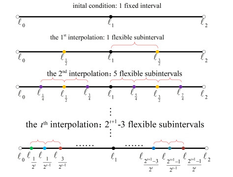
In the paper, the existence and uniqueness of the equilibrium point in the Cohen-Grossberg neural network (CGNN) are first studied. Additionally, a switched Cohen-Grossberg neural network (SCGNN) model with time-varying delay is established by introducing a switched system to the CGNN. Based on reducing the conservativeness of the system, a flexible terminal interpolation method is proposed. Using an adjustable parameter to divide the invariant time-delay interval into multiple adjustable terminal interpolation intervals $ (2^{\imath +1}-3) $, more moments when signals are transmitted slowly can be captured. To this end, a new Lyapunov-Krasovskii functional (LKF) is constructed, and the stability of SCGNN can be estimated. Using the LKF method, a quadratic convex inequality, linear matrix inequalities (LMIs) and ordinary differential equation theory, a new form of stability criterion is obtained and specific instances are given to prove the applicability of the new stability criterion.

References

[1]	C. I. Byrnes, F. D. Priscoli, A. Isidori, Output regulation of uncertain nonlinear systems, Boston: Birkhäuser, 1997. https://doi.org/10.1007/978-1-4612-2020-6
[2]	Z. H. Yuan, L. H. Huang, D. W. Hu, B. W. Liu, Convergence of nonautonomous Cohen-Grossberg-type neural networks with variable delays, IEEE Trans. Neural Netw., 19 (2008), 140-147. https://doi.org/10.1109/TNN.2007.903154 doi: 10.1109/TNN.2007.903154
[3]	H. Ye, A. N. Michel, K. N. Wang, Qualitative analysis of Cohen-Grossberg neural networks with multiple delays, Phys. Rev. E, 51 (1995), 2611. https://doi.org/10.1103/PhysRevE.51.2611 doi: 10.1103/PhysRevE.51.2611
[4]	J. D. Cao, K. Yuan, H. X. Li, Global asymoptotical stability of recurrent neural networks with multiple discrete delays and distributed delays, IEEE Trans. Neural Netw., 17 (2006), 1646-1651. https://doi.org/10.1109/TNN.2006.881488 doi: 10.1109/TNN.2006.881488
[5]	C. X. Huang, L. H. Huang, Dynamics of a class of Cohen-Grossberg neural networks with time-varying delays, Nonlinear Anal. Real World Appl., 8 (2007), 40-52. https://doi.org/10.1016/j.nonrwa.2005.04.008 doi: 10.1016/j.nonrwa.2005.04.008
[6]	J. D. Cao, J. L. Liang, Boundedness and stability for Cohen-Grossberg neural networks with time-varying delays, J. Math. Anal. Appl., 296 (2004), 665-685. https://doi.org/10.1016/j.jmaa.2004.04.039 doi: 10.1016/j.jmaa.2004.04.039
[7]	L. Wan, Q. H. Zhou, Attractor and ultimate boundedness for stochastic cellular neural networks with delays, Nonlinear Anal. Real World Appl., 12 (2011), 2561-2566. https://doi.org/10.1016/j.nonrwa.2011.03.005 doi: 10.1016/j.nonrwa.2011.03.005
[8]	K. Yuan, J. D. Cao, H. X. Li, Robust stability of switched Cohen-Grossberg neural networks with mixed time-varying delays, IEEE Trans. Syst. Man Cybernet. Part B (Cybernet.), 36 (2006), 1356-1363. https://doi.org/10.1109/TSMCB.2006.876819 doi: 10.1109/TSMCB.2006.876819
[9]	H. B. Zeng, H. C. Lin, Y. He, K. L. Teo, W. Wang, Hierarchical stability conditions for time-varying delay systems via an extended reciprocally convex quadratic inequality, J. Franklin Inst., 357 (2020), 9930-9941. https://doi.org/10.1016/j.jfranklin.2020.07.034 doi: 10.1016/j.jfranklin.2020.07.034
[10]	H. Y. Zhang, Z. P. Qiu, X. Z. Liu, L. L. Xiong, Stochastic robust finite-time boundedness for semi-Markov jump uncertain neutral-type neural networks with mixed time-varying delays via a generalized reciprocally convex combination inequality, Int. J. Robust Nonlinear Control, 30 (2020), 2001-2019. https://doi.org/10.1002/rnc.4859 doi: 10.1002/rnc.4859
[11]	W. J. Lin, Y. He, M. Wu, Q. P. Liu, Reachable set estimation for Markovian jump neural networks with time-varying delay, Neural Netw., 108 (2018), 527-532. https://doi.org/10.1016/j.neunet.2018.09.011 doi: 10.1016/j.neunet.2018.09.011
[12]	W. Y. Duan, Stability switches in a Cohen-Grossberg neural network with multi-delays, Int. J. Biomath., 10 (2017), 1750075. https://doi.org/10.1142/S1793524517500759 doi: 10.1142/S1793524517500759
[13]	D. Liberzon, Switching in system and control, Boston: Birkhäuser, 2003. https://doi.org/10.1007/978-1-4612-0017-8
[14]	J. Lian, K. Zhang, Exponential stability for switched Cohen-Grossberg neural networks with average dwell time, Nonlinear Dyn., 63 (2011), 331-343. https://doi.org/10.1007/s11071-010-9807-2 doi: 10.1007/s11071-010-9807-2
[15]	Z. G. Wu, P. Shi, H. Y. Su, J. Chu, Delay-dependent stability analysis for switched neural networks with time-verying delay, IEEE Trans. Syst. Man Cybernet. Part B (Cybernet.), 41 (2011), 1522-1530. https://doi.org/10.1109/TSMCB.2011.2157140 doi: 10.1109/TSMCB.2011.2157140
[16]	D. Liberzon, A. S. Morse, Basic problems in stability and design of switched systems, IEEE Control Syst. Mag., 19 (1999), 59-70. https://doi.org/10.1109/37.793443 doi: 10.1109/37.793443
[17]	Q. K. Song, J. Y. Zhang, Global exponential stability of impulsive Cohen-Grossberg neural network with time-varying delays, Nonlinear Anal. Real World Appl., 9 (2008), 500-510. https://doi.org/10.1016/j.nonrwa.2006.11.015 doi: 10.1016/j.nonrwa.2006.11.015
[18]	Q. T. Gan, Exponential synchronization of stochastic Cohen-Grossberg neural networks with mixed time-varying delays and reaction-diffusion via periodically intermittent control, Neural Netw., 31 (2012), 12-21. https://doi.org/10.1016/j.neunet.2012.02.039 doi: 10.1016/j.neunet.2012.02.039
[19]	M. H. Jiang, Y. Shen, X. X. Liao, Boundedness and global exponential stability for generalized Cohen-Grossberg neural networks with variable delay, Appl. Math. Comput., 172 (2006), 379-393. https://doi.org/10.1016/j.amc.2005.02.009 doi: 10.1016/j.amc.2005.02.009
[20]	L. G. Wan, A. L. Wu, Mittag-Leffler stability analysis of fractional-order fuzzy Cohen-Grossberg neural networks with deviating argument, Adv. Differ. Equ., 2017 (2017), 1-19. https://doi.org/10.1186/s13662-017-1368-y doi: 10.1186/s13662-017-1368-y
[21]	H. Q. Wu, G. H. Xu, C. Y. Wu, N. Li, K. W. Wang, Q. Q. Guo, Stability in switched Cohen-Grossberg neural networks with mixed time delays and non-Lipschitz activation functions, Discrete Dyn. Nat. Soc., 2012 (2012), 1-22. https://doi.org/10.1155/2012/435402 doi: 10.1155/2012/435402
[22]	B. Sun, Y. T. Cao, Z. Y. Guo, Z. Yan, S. P. Wen, Synchronization of discrete-time recurrent neural networks with time-varying delays via quantized sliding mode control, Appl. Math. Comput., 375 (2020), 125093. https://doi.org/10.1016/j.amc.2020.125093 doi: 10.1016/j.amc.2020.125093
[23]	Z. S. Wang, Y. F. Tian, Stability analysis of recurrent neural networks with time-varying delay by flexible terminal interpolation method, IEEE Trans. Neural Netw. Learn. Syst., 2022. https://doi.org/10.1109/TNNLS.2022.3188161
[24]	H. G. Zhang, Z. W. Liu, G. B. Huang, Z. S. Wang, Novel weighting-delay-based stability criteria for recurrent neural networks with time-varying delay, IEEE Trans. Neural Netw., 21 (2010), 91-106. https://doi.org/10.1109/TNN.2009.2034742 doi: 10.1109/TNN.2009.2034742
[25]	Y. He, G. P. Liu, D. Rees, New delay-dependent stability criteria for neural networks with time-varying delay, IEEE Trans. Neural Netw., 18 (2007), 310-314. https://doi.org/10.1109/TNN.2006.888373 doi: 10.1109/TNN.2006.888373
[26]	M. N. A. Parlakçı, Robust stability of uncertain neutral systems: a novel augmented Lyapunov functional approach, IET Control Theory Appl., 1 (2007), 802-809. https://doi.org/10.1049/iet-cta:20050517 doi: 10.1049/iet-cta:20050517
[27]	C. Peng, Y. C. Tian, Delay-dependent robust stability criteria for uncertain systems with interval time-varying delay, J. Comput. Appl. Math., 214 (2008), 480-494. https://doi.org/10.1016/j.cam.2007.03.009 doi: 10.1016/j.cam.2007.03.009
[28]	T. Li, L. Guo, C. Y. Sun, C. Lin, Further result on delay-dependent stability criterion of neural networks with time-varying delays, IEEE Trans. Neural Netw., 19 (2008), 726-730. https://doi.org/10.1109/TNN.2007.914162 doi: 10.1109/TNN.2007.914162
[29]	S. Arik, Z. Orman, Global stability analysis of Cohen-Grossberg neural networks with time varying delays, Phys. Lett. A, 341 (2005), 410-421. https://doi.org/10.1016/j.physleta.2005.04.095 doi: 10.1016/j.physleta.2005.04.095
[30]	Z. Y. Dong, X. Wang, X. Zhang, A nonsingular M-matrix-based global exponential stability analysis of higher-order delayed discrete-time Cohen-Grossberg neural networks, Appl. Math. Comput., 385 (2020), 125401. https://doi.org/10.1016/j.amc.2020.125401 doi: 10.1016/j.amc.2020.125401
[31]	V. Singh, Improved global robust stability for interval-delayed Hopfield neural networks, Neural Process. Lett., 27 (2008), 257-265. https://doi.org/10.1007/s11063-008-9074-0 doi: 10.1007/s11063-008-9074-0
[32]	G. Bao, S. P. Wen, Z. G. Zeng, Robust stability analysis of interval fuzzy Cohen-Grossberg neural networks with piecewise constant argument of generalized type, Neural Netw., 33 (2012), 32-41. https://doi.org/10.1016/j.neunet.2012.04.003 doi: 10.1016/j.neunet.2012.04.003
[33]	G. Q. Tan, Z. S. Wang, Reachable set estimation of delayed Markovian jump neural networks based on an improved reciprocally convex inequality, IEEE Trans. Neural Netw. Learn. Syst., 33 (2022), 2737-2742. https://doi.org/10.1109/TNNLS.2020.3045599 doi: 10.1109/TNNLS.2020.3045599
[34]	Z. J. Zhang, X. Zhang, T. T. Yu, Global exponential stability of neutral-type Cohen-Grossberg neural networks with multiple time-varying neutral and discrete delays, Neurocomputing, 490 (2022), 124-131. https://doi.org/10.1016/j.neucom.2022.03.068 doi: 10.1016/j.neucom.2022.03.068

Reader Comments

Your name:*

Email:*
© 2023 the Author(s), licensee AIMS Press. This is an open access article distributed under the terms of the Creative Commons Attribution License (http://creativecommons.org/licenses/by/4.0)