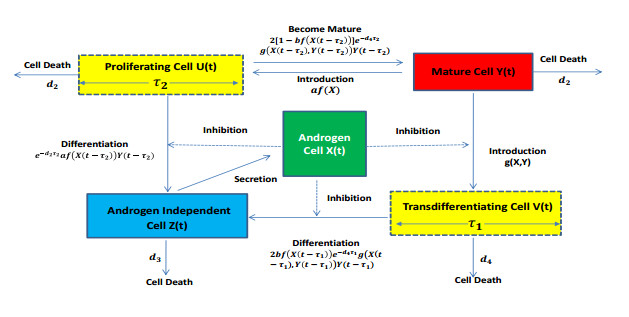
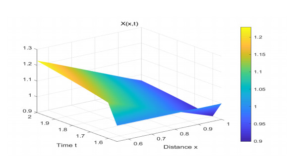
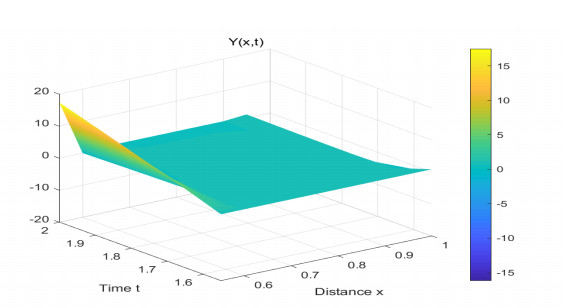
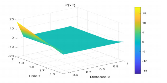
Prostate cancer is a serious disease that endangers men's health. The genetic mechanism and treatment of prostate cancer have attracted the attention of scientists. In this paper, we focus on the nonlinear mixed reaction diffusion dynamics model of neuroendocrine transdifferentiation of prostate cancer cells with time delays, and reveal the evolutionary mechanism of cancer cells mathematically. By applying operator semigroup theory and the comparison principle of parabolic equation, we study the global existence, uniqueness and boundedness of the positive solution for the model. Additionally, the global invariant set and compact attractor of the positive solution are obtained by Kuratowski's measure of noncompactness. Finally, we use the Pdepe toolbox of MATLAB to carry out numerical calculations and simulations on an example to check the correctness and effectiveness of our main results. Our results show that the delay has no effect on the existence, uniqueness, boundedness and invariant set of the solution, but will affect the attractor.
Citation: Kaihong Zhao. Attractor of a nonlinear hybrid reaction–diffusion model of neuroendocrine transdifferentiation of human prostate cancer cells with time-lags[J]. AIMS Mathematics, 2023, 8(6): 14426-14448. doi: 10.3934/math.2023737
Prostate cancer is a serious disease that endangers men's health. The genetic mechanism and treatment of prostate cancer have attracted the attention of scientists. In this paper, we focus on the nonlinear mixed reaction diffusion dynamics model of neuroendocrine transdifferentiation of prostate cancer cells with time delays, and reveal the evolutionary mechanism of cancer cells mathematically. By applying operator semigroup theory and the comparison principle of parabolic equation, we study the global existence, uniqueness and boundedness of the positive solution for the model. Additionally, the global invariant set and compact attractor of the positive solution are obtained by Kuratowski's measure of noncompactness. Finally, we use the Pdepe toolbox of MATLAB to carry out numerical calculations and simulations on an example to check the correctness and effectiveness of our main results. Our results show that the delay has no effect on the existence, uniqueness, boundedness and invariant set of the solution, but will affect the attractor.

| [1] | J. Horoszewicz, S. Leong, T. Ming-Chu, Z. L. Wajsman, M. Friedman, L. Papsidero, et al., The LNCaP cell line-A new model for studies on human prostatic carcinoma, Prog. Clin. Biol. Res., 37 (1980), 115–132. |
| [2] |
K. Swanson, L. True, D. Lin, K. R. Buhler, R. Vessella, J. D. Murray, A quantitative model for the dynamics of serum prostate-specific antigen as a marker for cancerous growth: an explanation for a medic anomaly, Am. J. Pathol., 163 (2001), 2513–2522. https://doi.org/10.1016/S0002-9440(10)64691-3 doi: 10.1016/S0002-9440(10)64691-3

|
| [3] |
R. T. Vollmer, S. Egaqa, S. Kuwao, S. Baba, The dynamics of prostate antigen during watchful waiting of prostate carcinoma: a study of 94 japanese men, Cancer, 94 (2002), 1692–1698. https://doi.org/10.1002/cncr.10443 doi: 10.1002/cncr.10443
|
| [4] | R. Vollmer, P. Humphrey, Tumor volume in prostate cancer and serum prostate-specific antigen: analysis from a kinetic viewpoint, Am. J. Pathol., 119 (2003), 80–89. |
| [5] | Y. Kuang, J. Nagy, J. Elser, Biological stoichiometry of tumor dynamics: mathematical models and analysis, Discrete Contin. Dyn. Syst. Ser. B, 4 (2004), 221–240. |
| [6] |
C. Heinlein, C. Chang, Androgen receptor in prostate cancer, Endocr. Rev., 25 (2004), 276–308. https://doi.org/10.1210/er.2002-0032 doi: 10.1210/er.2002-0032
|
| [7] | P. Koivisto, M. Kolmer, T. Visakorpi, O. P. Kallioniemi, Androgen receptor gene and hormonal therapy failure of prostate cancer, Am. J. Pathol., 152 (1998), 1–9. |
| [8] |
R. Rittmaster, A. Manning, A. Wright, L. N. Thomas, S. Whitefield, R. W. Norman, et al., Evidence for atrophy and apoptosis in the ventral prostate of rats given the 5 alpha-reductase inhibitor finasteride, Endocrinology, 136 (1995), 741–748. https://doi.org/10.1210/en.136.2.741 doi: 10.1210/en.136.2.741
|
| [9] |
T. Jackson, A mathematical investigation of the multiple pathways to recurrent prostate cancer: Comparison with experimental data, Neoplasia, 6 (2004), 697–704. https://doi.org/10.1593/neo.04259 doi: 10.1593/neo.04259
|
| [10] |
T. Jackson, A mathematical model of prostate tumor growth and androgen-independent relapse, Discrete Contin. Dyn. Syst. Ser. B, 4 (2004), 187–201. https://doi.org/10.3934/dcdsb.2004.4.187 doi: 10.3934/dcdsb.2004.4.187
|
| [11] |
A. Ideta, G. Tanaka, T. Takeuchi, K. Aihara, A mathematical model of intermittent androgen suppression for prostate cancer, J. Nonlinear Sci., 18 (2008), 593. https://doi.org/10.1007/s00332-008-9031-0 doi: 10.1007/s00332-008-9031-0
|
| [12] |
S. Eikenberry, J. Nagy, Y. Kuang, The evolutionary impact of androgen levels on prostate cancer in a multi-scale mathematical model, Biol. Direct., 5 (2010), 24. https://doi.org/10.1186/1745-6150-5-24 doi: 10.1186/1745-6150-5-24
|
| [13] |
S. Terry, H. Beltran, The many faces of neuroendocrine differentiation in prostate cancer progression, Front. Oncol., 4 (2014), 60. https://doi.org/10.3389/fonc.2014.00060 doi: 10.3389/fonc.2014.00060
|
| [14] |
M. Cerasuolo, D. Paris, F. Iannotti, D. Melck, R. Verde, E. Mazzarella, et al., Neuroendocrine transdifferentiation in human prostate cancer cells: an integrated approach, Cancer Res., 75 (2015), 2975–2986. https://doi.org/10.1158/0008-5472.CAN-14-3830 doi: 10.1158/0008-5472.CAN-14-3830
|
| [15] |
J. Morken, A. Packer, R. Everett, J. D. Nagy, Y, Kuang, Mechanisms of resistance to intermittent androgen deprivation in patients with prostate cancer identified by a novel computational method, Cancer Res., 74 (2014), 3673–3683. https://doi.org/10.1158/0008-5472.CAN-13-3162 doi: 10.1158/0008-5472.CAN-13-3162
|
| [16] |
L. Turner, A. Burbanks, M. Cerasuolo, Mathematical insights into neuroendocrine transdifferentiation of human prostate cancer cells, Nonlinear Anal. Model., 26 (2021), 884–913. https://doi.org/10.15388/namc.2021.26.24441 doi: 10.15388/namc.2021.26.24441
|
| [17] |
A. Rezounenko, Viral infection model with diffusion and distributed delay: finite-dimensional global attractor, Qual. Theor. Dyn. Syst., 22 (2023), 11. https://doi.org/10.1007/s12346-022-00707-6 doi: 10.1007/s12346-022-00707-6
|
| [18] |
O. Nave, M. Elbaz, Method of directly defining the inverse mapping applied to prostate cancer immunotherapy-mathematical model, Int. J. Biomath., 11 (2018), 1850072. https://doi.org/10.1142/s1793524518500729 doi: 10.1142/s1793524518500729
|
| [19] |
K. H. Zhao, Global stability of a novel nonlinear diffusion online game addiction model with unsustainable control, AIMS Math., 7 (2022), 20752–20766. https://doi.org/10.3934/math.20221137 doi: 10.3934/math.20221137
|
| [20] |
K. H. Zhao, Probing the oscillatory behavior of internet game addiction via diffusion PDE model, Axioms, 11 (2022), 649. https://doi.org/10.3390/axioms11110649 doi: 10.3390/axioms11110649
|
| [21] |
M. Adimy, F. Crauste, C. Marquet, Asymptotic behaviour and stability switch for a mature-immature model of cell differentiation, Nonlinear Anal. RWA., 11 (2010), 2913–2929. https://doi.org/10.1016/j.nonrwa.2009.11.001 doi: 10.1016/j.nonrwa.2009.11.001
|
| [22] |
M. Adimy, F. Crauste, S, Ruan, Modelling hematopoiesis mediated by growth factors with applications to periodic hematological diseases, Bull. Math. Biol., 68 (2006), 2321–2351. https://doi.org/10.1007/s11538-006-9121-9 doi: 10.1007/s11538-006-9121-9
|
| [23] | H. L. Smith, Monotone dynamical systems: an introduction to the theory of competitive and cooperative systems, Washington: American Mathematical Society, 1995. |
| [24] | R. Martin, H. L. Smith, Abstract functional differential equtions and reaction-diffusion systems, Trans. Amer. Math. Soc., 321 (1990), 1–44. |
| [25] |
Y. Lou, X. Zhao, A reaction-diffusion malaria model with incubation period in the vector population, J. Math. Biol., 62 (2011), 62,543–568. https://doi.org/10.1007/s00285-010-0346-8 doi: 10.1007/s00285-010-0346-8
|
| [26] | K. Deimling, Nonlinear functional analysis, Berlin: Springer Verlag, 1988. |
| [27] | G. Sell, Y. You, Dynamics of evolutionary equations, New York: Springer Verlag, 2002. |
| [28] |
P. Magal, X. Zhao, Global attractors and steady states for uniformly persistent dynamical systems, SIAM J. Math. Anal., 37 (2005), 251–275. https://doi.org/10.1137/S0036141003439173 doi: 10.1137/S0036141003439173
|
| [29] |
J. Gómez-Aguilar, M. López-López, V. Alvarado-Martínez, D. Baleanu, H. Khan, Chaos in a cancer model via fractional derivatives with exponential decay and Mittag-Leffler law, Entropy, 19 (2017), 681. https://doi.org/10.3390/e19120681 doi: 10.3390/e19120681
|
| [30] |
S. Kumar, A. Kumar, B. Samet, J. Gómez-Aguilar, M. S. Osman, A chaos study of tumor and effector cells in fractional tumor-immune model for cancer treatment, Chaos Soliton. Fract., 141 (2020), 110321. https://doi.org/10.1016/j.chaos.2020.110321 doi: 10.1016/j.chaos.2020.110321
|
| [31] |
K. H. Zhao, Stability of a nonlinear ML-nonsingular kernel fractional Langevin system with distributed lags and integral control, Axioms, 11 (2022), 350. https://doi.org/10.3390/axioms11070350 doi: 10.3390/axioms11070350
|
| [32] |
K. H. Zhao, Existence, stability and simulation of a class of nonlinear fractional Langevin equations involving nonsingular Mittag-Leffler kernel, Fractal Fract., 6 (2022), 469. https://doi.org/10.3390/fractalfract6090469 doi: 10.3390/fractalfract6090469
|
| [33] |
K. H. Zhao, Stability of a nonlinear fractional Langevin system with nonsingular exponential kernel and delay control, Discrete Dyn. Nat. Soc., 2022 (2022), 9169185. https://doi.org/10.1155/2022/9169185 doi: 10.1155/2022/9169185
|
| [34] |
K. H. Zhao, Coincidence theory of a nonlinear periodic Sturm-Liouville system and its applications, Axioms, 11 (2022), 726. https://doi.org/10.3390/axioms11120726 doi: 10.3390/axioms11120726
|
| [35] |
K. H. Zhao, Stability of a nonlinear Langevin system of ML-type fractional derivative affected by time-varying delays and differential feedback control, Fractal Fract., 6 (2022), 725. https://doi.org/10.3390/fractalfract6120725 doi: 10.3390/fractalfract6120725
|
| [36] |
H. Huang, K. H. Zhao, X. D. Liu, On solvability of BVP for a coupled Hadamard fractional systems involving fractional derivative impulses, AIMS Math., 7 (2022), 19221–19236. https://doi.org/10.3934/math.20221055 doi: 10.3934/math.20221055
|
| [37] |
K. H. Zhao, Existence and UH-stability of integral boundary problem for a class of nonlinear higher-order Hadamard fractional Langevin equation via Mittag-Leffler functions, Filomat, 37 (2023), 1053–1063. https://doi.org/10.2298/FIL2304053Z doi: 10.2298/FIL2304053Z
|
| [38] |
K. H. Zhao, Solvability and GUH-stability of a nonlinear CF-fractional coupled Laplacian equations, AIMS Math., 8 (2023), 13351–13367. https://doi.org/10.3934/math.2023676 doi: 10.3934/math.2023676
|
| [39] |
K. H. Zhao, Local exponential stability of four almost-periodic positive solutions for a classic Ayala-Gilpin competitive ecosystem provided with varying-lags and control terms, Int. J. Control, 2022. https://doi.org/10.1080/00207179.2022.2078425 doi: 10.1080/00207179.2022.2078425
|
| [40] |
K. H. Zhao, Local exponential stability of several almost periodic positive solutions for a classical controlled GA-predation ecosystem possessed distributed delays, Appl. Math. Comput., 437 (2023), 127540. https://doi.org/10.1016/j.amc.2022.127540 doi: 10.1016/j.amc.2022.127540
|
| [41] |
K. H. Zhao, Global exponential stability of positive periodic solutions for a class of multiple species Gilpin-Ayala system with infinite distributed time delays, Int. J. Control, 94 (2021), 521–533. https://doi.org/10.1080/00207179.2019.1598582 doi: 10.1080/00207179.2019.1598582
|
| [42] |
K. H. Zhao, Existence and stability of a nonlinear distributed delayed periodic AG-ecosystem with competition on time scales, Axioms, 12 (2023), 315. https://doi.org/10.3390/axioms12030315 doi: 10.3390/axioms12030315
|
Figures(6) / Tables(5)

Kaihong Zhao. Attractor of a nonlinear hybrid reaction–diffusion model of neuroendocrine transdifferentiation of human prostate cancer cells with time-lags[J]. AIMS Mathematics, 2023, 8(6): 14426-14448. doi: 10.3934/math.2023737


 DownLoad: