The implementation comparison between the Euler and trivial coupling schemes for achieving strong convergence

Yousef Alnafisah; Yousef Alnafisah

doi:10.3934/math.20231520

AIMS Mathematics

2023, Volume 8, Issue 12: 29701-29712. doi: 10.3934/math.20231520

Previous Article Next Article

Research article

The implementation comparison between the Euler and trivial coupling schemes for achieving strong convergence

Yousef Alnafisah ^,

Department of Mathematics, College of Science, Qassim University, P.O. Box 6644, Buraydah 51452, Saudi Arabia

Received: 23 July 2023 Revised: 02 October 2023 Accepted: 23 October 2023 Published: 02 November 2023
MSC : 34C10, 34K11

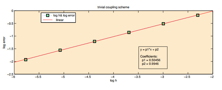
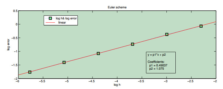
This study aimed to develop efficient numerical techniques with the same accuracy level as exact solutions of stochastic differential equations (SDEs). The MATLAB program was used to find solutions for the Euler and trivial coupling methods. The results of these methods were then compared and analyzed. The results show that Euler and trivial coupling methods give the same strong convergence. Furthermore, we demonstrated that these methods achieve strong convergence with a standard order of one-half to the exact solution of the SDE. Moreover, the Euler method is characterized by its speed, ease of application and ability to find solutions through computer programs.
- stochastic differential equations (SDEs),
- differential equations,
- trivial coupling method,
- Euler method,
- numerical solutions
Citation: Yousef Alnafisah. The implementation comparison between the Euler and trivial coupling schemes for achieving strong convergence[J]. AIMS Mathematics, 2023, 8(12): 29701-29712. doi: 10.3934/math.20231520

Related Papers:

Abstract

This study aimed to develop efficient numerical techniques with the same accuracy level as exact solutions of stochastic differential equations (SDEs). The MATLAB program was used to find solutions for the Euler and trivial coupling methods. The results of these methods were then compared and analyzed. The results show that Euler and trivial coupling methods give the same strong convergence. Furthermore, we demonstrated that these methods achieve strong convergence with a standard order of one-half to the exact solution of the SDE. Moreover, the Euler method is characterized by its speed, ease of application and ability to find solutions through computer programs.

References

[1]	L. Bachelier, Théorie de la spéculation, Ann. Sci. l'École Norm. S., Sér. 3, 17 (1900), 21–86. https://doi.org/10.24033/asens.476 doi: 10.24033/asens.476
[2]	A. Einstein, Zur theorie der brownschen Bewegung, Ann. Phys. IVAnn. Phys. IV, 19 (1906), 371–381.
[3]	N. Wiener, Differential space, J. Math. Phys., 2 (1923), 131–174. https://doi.org/10.1002/sapm192321131 doi: 10.1002/sapm192321131
[4]	K. Ito, Stochastic integral, Proc. Imp. Acad., 20 (1944), 519–524. https://doi.org/10.3792/pia/1195572786 doi: 10.3792/pia/1195572786
[5]	E. Allen, Modeling with Itô stochastic differential equations, Mathematical Modelling: Theory and Applications, Vol. 22, 2007. https://doi.org/10.1007/978-1-4020-5953-7
[6]	M. Carletti, K. Burrage, P. M. Burrage, Numerical simulation of stochastic ordinary differential equations in biomathematical modelling, Math. Comput. Simul., 64 (2004), 271–277.
[7]	A. Tocino, R. Ardanuy, Runge–Kutta methods for numerical solution of stochastic differential equations, J. Comput. Appl. Math., 138 (2002), 219–241. https://doi.org/10.1016/S0377-0427(01)00380-6 doi: 10.1016/S0377-0427(01)00380-6
[8]	R. Farnoosh, H. Rezazadeh, A. Sobhani, M. Behboudi, Analytical solutions for stochastic differential equations via martingale processes, Math. Sci., 9 (2015), 87–92. https://doi.org/10.1007/s40096-015-0153-x doi: 10.1007/s40096-015-0153-x
[9]	Q. Zhan, Mean-square numerical approximations to random periodic solutions of stochastic differential equations, Adv. Differ. Equ., 2015 (2015), 292. https://doi.org/10.1186/s13662-015-0626-0 doi: 10.1186/s13662-015-0626-0
[10]	Z. Yin, S. Gan, An improved Milstein method for stiff stochastic differential equations, Adv. Differ. Equ., 2015 (2015), 369. https://doi.org/10.1186/s13662-015-0699-9 doi: 10.1186/s13662-015-0699-9
[11]	P. E. Kloeden, E. Platen, Numerical solution of stochastic differential equations, Springer-Verlag, 1995.
[12]	M. Wiktorsson, Joint characteristic function and simultaneous simulation of iterated Itô integrals for multiple independent Brownian motions, Ann. Appl. Probab., 11 (2001), 470–487. https://doi.org/10.1214/aoap/1015345301 doi: 10.1214/aoap/1015345301
[13]	T. Rydén, M. Wiktrosson, On the simulation of iteraled Itô integrals, Stoch. Proc. Appl., 91 (2001), 151–168. https://doi.org/10.1016/S0304-4149(00)00053-3 doi: 10.1016/S0304-4149(00)00053-3
[14]	A. M. Davie, Pathwise approximation of stochastic differential equations using coupling, Preprint, 2014. Available from: http://www.maths.ed.ac.uk/ adavie/coum.pdf.
[15]	S. Kanagawa, The rate of convergence for approximate solutions of stochastic differential equations, Tokyo J. Math., 12 (1989), 33–48. https://doi.org/10.3836/tjm/1270133546 doi: 10.3836/tjm/1270133546
[16]	N. Fournier, Simulation and approximation of Lévy-driven stochastic differential equations, ESIAM: PS, 15 (2011), 233–248. https://doi.org/10.1051/ps/2009017 doi: 10.1051/ps/2009017
[17]	S. T. Rachev, L. Rüschendorff, Mass transportation problems, Volume 1: Theory, New York: Springer-Verlag, 1998. https://doi.org/10.1007/b98893
[18]	E. Rio, Upper bounds for minimal distances in the central limit theorem, Ann. Inst. Henri Poincaré Probab. Stat., 45 (2009), 802–817. https://doi.org/10.1214/08-AIHP187 doi: 10.1214/08-AIHP187
[19]	E. Rio, Asymptotic constants for minimal distances in the central limit theorem, Electron. Commun. Probab., 16 (2011), 96–103. https://doi.org/10.1214/ECP.v16-1609 doi: 10.1214/ECP.v16-1609
[20]	B. Charbonneau, Y. Svyrydov, P. F. Tupper, Weak convergence in the Prokhorov metric of methods for stochastic differential equations, IMA J. Numer. Anal., 30 (2010), 579–594. https://doi.org/10.1093/imanum/drn067 doi: 10.1093/imanum/drn067
[21]	L. N. Vasershtein, Markov processes over denumerable products of spaces describing large system of automata, Probl. Inform. Transm., 5 (1969), 64–72.
[22]	I. Gyöngy, N. Krylov, Existence of strong solutions for Itô's stochastic equations via approximations, Probab. Th. Rel. Fields, 105 (1996), 143–158. https://doi.org/10.1007/BF01203833 doi: 10.1007/BF01203833
[23]	A. Davie, KMT theory applied to approximations of SDE, In: D. Crisan, B. Hambly, T. Zariphopoulou, Stochastic analysis and applications 2014, Cham: Springer, 100 (2014), 185–201. https://doi.org/10.1007/978-3-319-11292-3_7
[24]	Y. Alnafisah, A new order from the combination of exact coupling and the Euler scheme, AIMS Math., 7 (2022), 6356–6364.
[25]	Y. Alnafisah, Multilevel MC method for weak approximation of stochastic differential equation with the exact coupling scheme, Open Math., 20 (2022), 305–312. https://doi.org/10.1515/math-2022-0019 doi: 10.1515/math-2022-0019
[26]	Y. Alnafisah, Comparison between Milstein and exact coupling methods using MATLAB for a particular two-dimensional stochastic differential equation, J. Inf. Sci. Eng., 36 (2020), 1223–1232. https://doi.org/10.6688/JISE.202011_36(6).0006 doi: 10.6688/JISE.202011_36(6).0006

Reader Comments

Your name:*

Email:*
© 2023 the Author(s), licensee AIMS Press. This is an open access article distributed under the terms of the Creative Commons Attribution License (http://creativecommons.org/licenses/by/4.0)