Finite difference schemes for time-dependent convection <i>q</i>-diffusion problem

Yasir Nawaz; Muhammad Shoaib Arif; Kamaleldin Abodayeh; Mairaj Bibi; Yasir Nawaz; Muhammad Shoaib Arif; Kamaleldin Abodayeh; Mairaj Bibi

doi:10.3934/math.2022897

AIMS Mathematics

2022, Volume 7, Issue 9: 16407-16421. doi: 10.3934/math.2022897

Previous Article Next Article

Research article

Finite difference schemes for time-dependent convection q-diffusion problem

1.
Department of Mathematics, Air University, PAF Complex E-9, Islamabad, 44000, Pakistan
2.
Department of Mathematics and Sciences, College of Humanities and Sciences, Prince Sultan University, Riyadh, Saudi Arabia
3.
Stochastic Analysis and Optimization Research Group, Department of Mathematics, Air University, PAF Complex E-9, Islamabad, 44000, Pakistan
4.
Department of Mathematics, Comsats University Islamabad, Park Road, Islamabad, 45550, Pakistan

Received: 13 April 2022 Revised: 31 May 2022 Accepted: 07 June 2022 Published: 06 July 2022
MSC : 65Mxx, 76Rxx

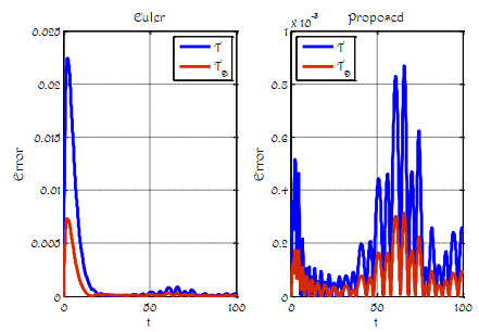
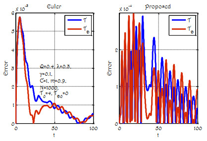
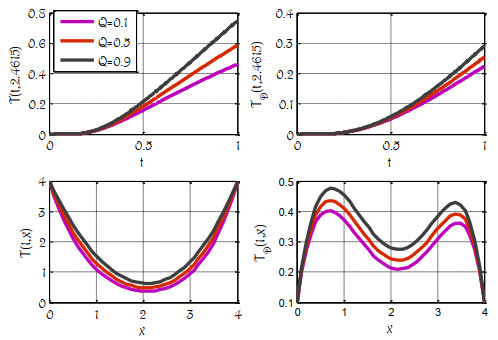
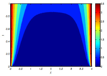
The energy balance ordinary differential equations (ODEs) model of climate change is extended to the partial differential equations (PDEs) model with convections and q-diffusions. Instead of integer order second-order partial derivatives, partial q-derivatives are considered. The local stability analysis of the ODEs model is established using the Routh-Hurwitz criterion. A numerical scheme is constructed, which is explicit and second-order in time. For spatial derivatives, second-order central difference formulas are employed. The stability condition of the numerical scheme for the system of convection q-diffusion equations is found. Both types of ODEs and PDEs models are solved with the constructed scheme. A comparison of the constructed scheme with the existing first-order scheme is also made. The graphical results show that global mean surface and ocean temperatures escalate by varying the heat source parameter. Additionally, these newly established techniques demonstrate predictability.
- energy balance model,
- convection and q-diffusion,
- heat source,
- second-order scheme,
- stability
Citation: Yasir Nawaz, Muhammad Shoaib Arif, Kamaleldin Abodayeh, Mairaj Bibi. Finite difference schemes for time-dependent convection q-diffusion problem[J]. AIMS Mathematics, 2022, 7(9): 16407-16421. doi: 10.3934/math.2022897

Related Papers:

Abstract

The energy balance ordinary differential equations (ODEs) model of climate change is extended to the partial differential equations (PDEs) model with convections and q-diffusions. Instead of integer order second-order partial derivatives, partial q-derivatives are considered. The local stability analysis of the ODEs model is established using the Routh-Hurwitz criterion. A numerical scheme is constructed, which is explicit and second-order in time. For spatial derivatives, second-order central difference formulas are employed. The stability condition of the numerical scheme for the system of convection q-diffusion equations is found. Both types of ODEs and PDEs models are solved with the constructed scheme. A comparison of the constructed scheme with the existing first-order scheme is also made. The graphical results show that global mean surface and ocean temperatures escalate by varying the heat source parameter. Additionally, these newly established techniques demonstrate predictability.

References

[1]	F. H. Jackson, XI.—On q-functions and a certain difference operator, Trans. R. Soc. Edinburgh, 46 (1909), 253-281. https://doi.org/10.1017/S0080456800002751 doi: 10.1017/S0080456800002751
[2]	T. Ernst, The history of q-calculus and a new method, Licentiate thesis, Uppsala University, 2001.
[3]	V. Kac, P. Cheung, Quantum calculus, New York: Springer, 2002. https://doi.org/10.1007/978-1-4613-0071-7
[4]	W. Siegel, Introduction to string field theory, Teaneck: World Scientific, 1988.
[5]	M. H. Annaby, Z. S. Mansour, q-fractional calculus and equations, Berlin, Heidelberg: Springer, 2012. https://doi.org/10.1007/978-3-642-30898-7
[6]	R. P. Agarwal, Certain fractional q-integrals and q-derivatives, Math. Proc. Cambridge Philos. Soc., 66 (1969), 365-370. https://doi.org/10.1017/S0305004100045060 doi: 10.1017/S0305004100045060
[7]	A. Aral, V. Gupta, R. P. Agarwal, Applications of q-calculus in operator theory, New York: Springer, 2013. https://doi.org/10.1007/978-1-4614-6946-9
[8]	W. H. Abdi, On q-Laplace transforms, Proc. Nat. Acad. Sci. India Sect. A, 29 (1960), 389-408.
[9]	W. H. Abdi, Application of q-Laplace transform to the solution of certain q-integral equations, Rend. Circ. Mat. Palermo, 11 (1962), 245-257. https://doi.org/10.1007/BF02843870 doi: 10.1007/BF02843870
[10]	M. H. Annaby, Z. S. Mansour, q-Taylor and interpolation series for Jackson q-difference operators, J. Math. Anal. Appl., 334 (2008), 472-483. https://doi.org/10.1016/j.jmaa.2008.02.033 doi: 10.1016/j.jmaa.2008.02.033
[11]	R. Askey, The q-gamma and q-beta functions, Appl. Anal., 8 (1978), 125-141. https://doi.org/10.1080/00036817808839221 doi: 10.1080/00036817808839221
[12]	G. E. Andrews, R. Askey, R. Roy, Special functions, Cambridge: Cambridge University Press, 1999. https://doi.org/10.1017/CBO9781107325937
[13]	T. Abdeljawad, J. Alzabut, D. Baleanu, A generalized q-fractional Gronwall inequality and its applications to nonlinear delay q-fractional difference systems, J. Inequal. Appl., 2016 (2016), 240. https://doi.org/10.1186/s13660-016-1181-2 doi: 10.1186/s13660-016-1181-2
[14]	H. Aktuglu, M. A. Özarslan, On the solvability of Caputo q-fractional boundary value problem involving p-Laplacian operator, Abstr. Appl. Anal., 2013 (2013), 658617. http://doi.org/10.1155/2013/658617 doi: 10.1155/2013/658617
[15]	J. Ren, C. B. Zhai, Nonlocal q-fractional boundary value problem with Stieltjes integral conditions, Nonlinear Anal. Model., 24 (2019), 582-602. https://doi.org/10.15388/NA.2019.4.6 doi: 10.15388/NA.2019.4.6
[16]	T. Zhang, Q. X. Guo, The solution theory of the nonlinear q-fractional differential equations, Appl. Math. Lett., 104 (2020), 106282. https://doi.org/10.1016/j.aml.2020.106282 doi: 10.1016/j.aml.2020.106282
[17]	T. Zhang, Y. Z. Wang, The unique existence of solution in the q-integrable space for the nonlinear q-fractional differential equations, Fractals, 29 (2021), 2150050. https://doi.org/10.1142/S0218348X2150050X doi: 10.1142/S0218348X2150050X
[18]	M. A. Alqudah, A. Kashuri, P. O. Mohammed, T. Abdeljawad, M. Raees, M. Anwar, et al., Hermite-Hadamard integral inequalities on coordinated convex functions in quantum calculus, Adv. Differ. Equ. 2021 (2021), 264. https://doi.org/10.1186/s13662-021-03420-x doi: 10.1186/s13662-021-03420-x
[19]	A. Eryılmaz, Spectral analysis of q-Sturm-Liouville problem with the spectral parameter in the boundary condition, J. Funct. Space, 2012 (2012), 736437. https://doi.org/10.1155/2012/736437 doi: 10.1155/2012/736437
[20]	T. H. Koornwinder, R. F. Swarttouw, On q-analogues of the Fourier and Hankel transforms, T. Am. Math. Soc., 333 (1992), 445-461. https://doi.org/10.2307/2154118 doi: 10.2307/2154118
[21]	S. C. Jing, H. Y. Fan, q-Taylor's formula with its q-remainder, Commun. Theor. Phys., 23 (1995), 117-120. https://doi.org/10.1088/0253-6102/23/1/117 doi: 10.1088/0253-6102/23/1/117
[22]	T. Ernst, A method for q-calculus, J. Nonlinear Math. Phys., 10 (2003), 487-525. https://doi.org/10.2991/jnmp.2003.10.4.5 doi: 10.2991/jnmp.2003.10.4.5
[23]	P. Singh, P. K. Mishra, R. S. Pathak, q-iterative methods, IOSR-JM, 9 (2013), 6-10.
[24]	H. Jafari, S. J. Johnston, S. M. Sani, D. Baleanu, A decomposition method for solving q-difference equations, Appl. Math. Inf. Sci., 9 (2015), 2917-2920. http://doi.org/10.12785/amis/090618 doi: 10.12785/amis/090618
[25]	J. Lin, Simulation of 2D and 3D inverse source problems of nonlinear time-fractional wave equation by the meshless homogenization function method, Eng. Comput., 2021. https://doi.org/10.1007/s00366-021-01489-2 doi: 10.1007/s00366-021-01489-2
[26]	A. O. Ahmet, S. I. Butt, M. Nadeem, M. A. Ragusa, New general variants of Chebyshev type inequalities via generalized fractional integral operators, Mathematics, 9 (2021), 122. https://doi.org/10.3390/math9020122 doi: 10.3390/math9020122
[27]	S. Kızıla, M. A. Ardıc, Inequalities for strongly convex functions via Atangana-Baleanu integral operators, Turk. J. Sci., 6 (2021), 96-109.
[28]	December 2018 Global Climate Report, National Centers for Environmental Information, 2018. Available from: https://www.ncei.noaa.gov/access/monitoring/monthly-report/global/201812.
[29]	M. I. Budyko, The effect of solar radiation variations on the climate of the Earth, Tellus., 21 (1969), 611-619. https://doi.org/10.3402/tellusa.v21i5.10109 doi: 10.3402/tellusa.v21i5.10109
[30]	W. D. Sellers, A global climatic model based on the energy balance of the Earth atmosphere system, J. Appl. Meteorol. Clim., 8 (1969), 392-400. https://doi.org/10.1175/1520-0450(1969)008 < 0392:AGCMBO > 2.0.CO; 2 doi: 10.1175/1520-0450(1969)008<0392:AGCMBO>2.0.CO;2
[31]	G. Sana, P. O. Mohammed, D. Y. Shin, M. A. Noor, M. S. Oudat, On iterative methods for solving nonlinear equations in Quantum calculus, Fractal Fract., 5 (2021), 60. https://doi.org/10.3390/fractalfract5030060 doi: 10.3390/fractalfract5030060
[32]	A. M. Wazwaz, Partial differential equations and solitary waves theory, Berlin, Heidelberg: Springer, 2009. http://doi.org/10.1007/978-3-642-00251-9
[33]	Y. Nawaz, M. S. Arif, K. Abodayeh, An explicit-implicit numerical scheme for time fractional boundary layer flows, Int. J. Numer. Meth. Fluids., 97 (2022), 920-940. https://doi.org/10.1002/fld.5078 doi: 10.1002/fld.5078
[34]	Y. Nawaz, M. S. Arif, W. Shatanawi, A new numerical scheme for time fractional diffusive SEAIR model with non-linear incidence rate: An application to computational biology, Fractal Fract., 6 (2022), 78. https://doi.org/10.3390/fractalfract6020078 doi: 10.3390/fractalfract6020078
[35]	Y. Nawaz, M. S. Arif, W. Shatanawi, M. U. Ashraf, A new unconditionally stable implicit numerical scheme for fractional diffusive epidemic model, AIMS Mathematics, 7 (2022), 14299-14322. https://doi.org/10.3934/math.2022788 doi: 10.3934/math.2022788

Reader Comments

Your name:*

Email:*
© 2022 the Author(s), licensee AIMS Press. This is an open access article distributed under the terms of the Creative Commons Attribution License (http://creativecommons.org/licenses/by/4.0)