Approximate solutions of the $ 2 $D space-time fractional diffusion equation via a gradient-descent iterative algorithm with Grünwald-Letnikov approximation

Adisorn Kittisopaporn; Pattrawut Chansangiam; Adisorn Kittisopaporn; Pattrawut Chansangiam

doi:10.3934/math.2022472

AIMS Mathematics

2022, Volume 7, Issue 5: 8471-8490. doi: 10.3934/math.2022472

Previous Article Next Article

Research article Special Issues

Approximate solutions of the $ 2 $D space-time fractional diffusion equation via a gradient-descent iterative algorithm with Grünwald-Letnikov approximation

Department of Mathematics, School of Science, King Mongkut's Institute of Technology Ladkrabang, Bangkok 10520, Thailand

Received: 31 December 2021 Revised: 12 February 2022 Accepted: 21 February 2022 Published: 28 February 2022
MSC : 65F10, 65N22, 34A08, 15A60

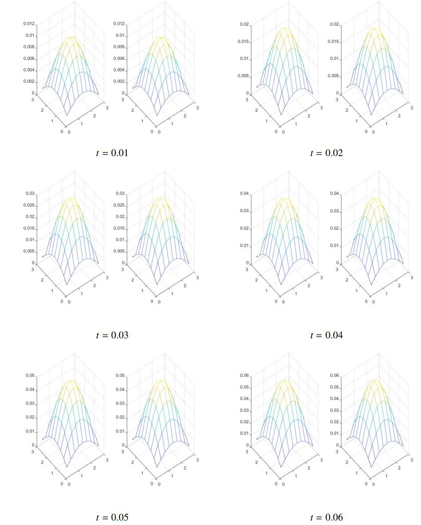
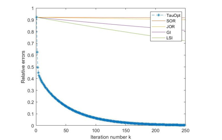
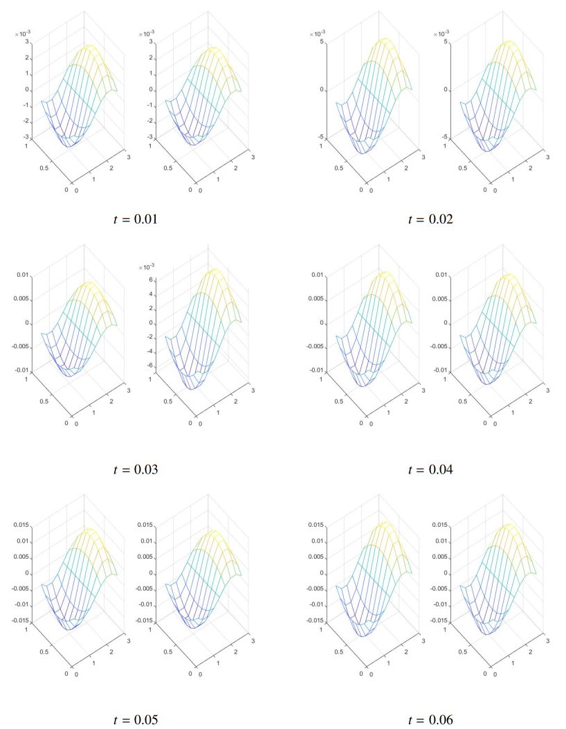
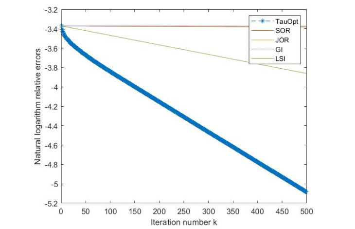
We consider the two-dimensional space-time fractional differential equation with the Caputo's time derivative and the Riemann-Liouville space derivatives on bounded domains. The equation is subjected to the zero Dirichlet boundary condition and the zero initial condition. We discretize the equation by finite difference schemes based on Grünwald-Letnikov approximation. Then we linearize the discretized equations into a sparse linear system. To solve such linear system, we propose a gradient-descent iterative algorithm with a sequence of optimal convergence factor aiming to minimize the error occurring at each iteration. The convergence analysis guarantees the capability of the algorithm as long as the coefficient matrix is invertible. In addition, the convergence rate and error estimates are provided. Numerical experiments demonstrate the efficiency, the accuracy and the performance of the proposed algorithm.
- fractional derivatives,
- fractional diffusion equation,
- Grünwald-Letnikov approximation,
- gradient descent,
- iterative method
Citation: Adisorn Kittisopaporn, Pattrawut Chansangiam. Approximate solutions of the $ 2 $D space-time fractional diffusion equation via a gradient-descent iterative algorithm with Grünwald-Letnikov approximation[J]. AIMS Mathematics, 2022, 7(5): 8471-8490. doi: 10.3934/math.2022472

Related Papers:

Abstract

We consider the two-dimensional space-time fractional differential equation with the Caputo's time derivative and the Riemann-Liouville space derivatives on bounded domains. The equation is subjected to the zero Dirichlet boundary condition and the zero initial condition. We discretize the equation by finite difference schemes based on Grünwald-Letnikov approximation. Then we linearize the discretized equations into a sparse linear system. To solve such linear system, we propose a gradient-descent iterative algorithm with a sequence of optimal convergence factor aiming to minimize the error occurring at each iteration. The convergence analysis guarantees the capability of the algorithm as long as the coefficient matrix is invertible. In addition, the convergence rate and error estimates are provided. Numerical experiments demonstrate the efficiency, the accuracy and the performance of the proposed algorithm.

References

[1]	I. Podlubny, Fractional differential equations: An introduction to fractional derivatives, fractional differential equations, to methods of their solution and some of their applications, New York: Academic Press, 1998.
[2]	I. Podlubny, Fractional differential equations, New York: Academic Press, 1999.
[3]	R. Hilfer, Applications of fractional calculus in physics, Singapore: World Scientific Publishing, 2000.
[4]	V. V. Kulish, J. L. Lage, Application of fractional calculus to fluid mechanics, J. Fluids Eng., 124 (2002), 803–806. http://dx.doi.org/10.1115/1.1478062 doi: 10.1115/1.1478062
[5]	X. J. Jiang, P. J. Scott, Free-form surface filtering using the diffusion equation, Adv. Metrol., 2020,129–142. https://doi.org/10.1016/B978-0-12-821815-0.00006-X
[6]	Q. Liu, F. Liu, I. Turner, V. Anh, Approximation of the Levy-Feller advection-dispersion process by random walk and flnite difierence method, J. Comput. Phys., 222 (2007), 57–70.
[7]	P. Zhuang, F. Liu, Implicit difference approximation for the two-dimensional space-time fractional diffusion equation, J. Appl. Math. Comput., 25 (2007), 269–282.
[8]	J. Huang, F. Liu, The space-time fractional diffusion equation with Caputo derivatives, J. Appl. Math. Comput., 19 (2005), 179–190.
[9]	Z. Q. Chen, M. M. Meerschaert, E. Nane, Space-time fractional diffusion on bounded domains, J. Math. Anal. Appl., 393 (2012), 479–488. http://dx.doi.org/10.1016/j.jmaa.2012.04.032 doi: 10.1016/j.jmaa.2012.04.032
[10]	J. Mua, B. Ahmad, S. Huang, Existence and regularity of solutions to time-fractional diffusion equations, Comput. Math. Appl., 73 (2017), 985–996. https://doi.org/10.1016/j.camwa.2016.04.039 doi: 10.1016/j.camwa.2016.04.039
[11]	M. M. Meerschaert, D. A. Benson, H. P. Scheffler, B. Baeumer, Stochastic solution of space-time fractional diffusion equations, Phys. Rev. E, 65 (2002), 041103. http://dx.doi.org/10.1103/PhysRevE.65.041103 doi: 10.1103/PhysRevE.65.041103
[12]	L. Chen, R. H. Nochetto, E. Otárola, A. J. Salgado, A PDE approach to fractional diffusion: A posteriori error analysis, J. Comput. Phys., 293 (2015), 339–358. http://dx.doi.org/10.1016/j.jcp.2015.01.001 doi: 10.1016/j.jcp.2015.01.001
[13]	R. H. Nochetto, E. Otarola, A. J. Salgado, A PDE approach to fractional diffusion in general domains: A prior error analysis, Found. Comput. Math., 15 (2015), 733–791. http://dx.doi.org/10.1007/s10208-014-9208-x doi: 10.1007/s10208-014-9208-x
[14]	R. Gorenflo, F. Mainardi, Random walk models for space-fractional diffusion processes, Fract. Calc. Appl. Anal., 1 (1998), 167–191.
[15]	R. Gorenflo, F. Mainardi, Approximation of Lévy-Feller diffusion by random walk, Z. für Anal. Anwend., 18 (1999), 231–246. http://dx.doi.org/10.4171/ZAA/879 doi: 10.4171/ZAA/879
[16]	R. Gorenflo, F. Mainardi, M. P. Paradisi, Time fractional diffusion: A discrete random walk approach, Nonlinear Dyn., 29 (2002), 129–143. http://dx.doi.org/10.1023/A:1016547232119 doi: 10.1023/A:1016547232119
[17]	R. Gorenflo, F. Mainardi, D. Moretti, G. Pagnini, P. Paradisi, Discrete random walk models for space-time fractional diffusion, Chem. Phys., 284 (2002), 521–541. http://dx.doi.org/10.1016/S0301-0104(02)00714-0 doi: 10.1016/S0301-0104(02)00714-0
[18]	R. L. Magin, O. Abdullah, D. Baleanu, X. J. Zhou, Anomalous diffusion expressed through fractional order differential operators in the Bloch-Torrey equation, J. Magn. Reson., 190 (2008), 255–270. http://dx.doi.org/10.1016/j.jmr.2007.11.007 doi: 10.1016/j.jmr.2007.11.007
[19]	A. V. Chechkin, R. Gorenflo, I. M. Sokolov, Fractional diffusion in inhomogeneous media, J. Phys. Math. Gen., 38 (2005), 679–684. http://dx.doi.org/10.1088/0305-4470/38/42/L03 doi: 10.1088/0305-4470/38/42/L03
[20]	F. Santamaria, S. Wils, E. D. Schutter, G. J. Augustine, Anomalous diffusion in Purkinje cell dendrites caused by spines, Neuron, 52 (2006), 635–648. http://dx.doi.org/10.1016/j.neuron.2006.10.025 doi: 10.1016/j.neuron.2006.10.025
[21]	S. Umarov, S. Steinberg, Variable order differential equations with piecewise constant order-function and diffusion with changing modes, Z. für Anal. Anwend., 28 (2009), 431–450. https://doi.org/10.1016/j.poly.2008.11.015 doi: 10.1016/j.poly.2008.11.015
[22]	M. Inc, The approximate and exact solutions of the space and time-fractional Burgers equations with initial conditions by variational iteration method, J. Math. Anal. Appl., 345 (2008), 476–484. https://doi.org/10.1016/j.jmaa.2008.04.007 doi: 10.1016/j.jmaa.2008.04.007
[23]	N. H. Sweilam, M. M. Khader, R. F. Al-Bar, Numerical studies for a multi-order fractional differential equation, Phys. Lett. A, 371 (2007), 26–33. https://doi.org/10.1016/j.physleta.2007.06.016 doi: 10.1016/j.physleta.2007.06.016
[24]	L. Song, H. Zhang, Application of homotopy analysis method to fractional KdV-Burgers-KURamoto equation, Phys. Lett. A, 367 (2007), 88–94. https://doi.org/10.1016/j.physleta.2007.02.083 doi: 10.1016/j.physleta.2007.02.083
[25]	H. Jafari, V. Daftardar-Gejji, Solving linear and nonlinear fractional diffusion and wave equations by Adomian decomposition, Appl. Math.Comput., 180 (2006), 488–497. https://doi.org/10.1016/j.amc.2005.12.031 doi: 10.1016/j.amc.2005.12.031
[26]	C. Yang, J. Hou, An approximate solution of nonlinear fractional differential equation by Laplace transform and Adomian polynomials, J. Inf. Comput. Sci., 10 (2013), 213–222.
[27]	T. Akram, M. Abbas, A. I. Ismail, An extended cubic B-spline collocation scheme for time fractional sub-diffusion equation, AIP Conference Proceedings, 2019. https://doi.org/10.1063/1.5136449
[28]	T. Akram, M. Abbas, A. I. Ismail, Numerical solution of fractional cable equation via extended cubic B-spline, AIP Conference Proceedings, 2019. https://doi.org/10.1063/1.5121041
[29]	U. Ali, A. Iqbal, M. Sohail, F. A. Abdull, Z. Khan, Compact implicit difference approximation for time-fractional diffusion-wave equation, Alex. Eng. J., 61 (2022), 4119–4126. https://doi.org/10.1016/j.aej.2021.09.005 doi: 10.1016/j.aej.2021.09.005
[30]	A. Iqbal, M. J. Siddiqui, I. Muhia, M. Abbasb, T. Akram, Nonlinear waves propagation and stability analysis for planar waves at far field using quintic B-spline collocation method, Alex. Eng. J., 59 (2020), 2695–2703. https://doi.org/10.1016/j.aej.2020.05.011 doi: 10.1016/j.aej.2020.05.011
[31]	M. Syam, M. A. Refai, Solving fractional diffusion equation via the collocation method based on fractional Legendre functions, J. Comput. Meth. Phys., 381074, 2014. http://dx.doi.org/10.1155/2014/381074
[32]	M. R. Cui, Compact finite difference method for the fractional diffusion equation, J. Comput. Phys., 228 (2009), 7792–7804. http://dx.doi.org/10.1016/j.jcp.2009.07.021 doi: 10.1016/j.jcp.2009.07.021
[33]	K. Diethelm, J. M. Ford, N. J. Fordc, M. Weilbeer, Pitfalls in fast numerical solvers for fractional differential equations, J. Comput. Appl. Math., 186 (2006), 482–503. http://dx.doi.org/10.1016/j.cam.2005.03.023 doi: 10.1016/j.cam.2005.03.023
[34]	R. Du, W. R. Cao, Z. Z. Sun, A compact difference scheme for the fractional diffusion-wave equation, Appl. Math. Model., 34 (2010), 2998–3007. http://dx.doi.org/10.1016/j.apm.2010.01.008 doi: 10.1016/j.apm.2010.01.008
[35]	P. Kumar, O. P. Agrawal, Numerical scheme for the solution of fractional differential equations of order greater than one, J. Comput. Nonlin. Dyn., 1 (2006), 178–185. http://dx.doi.org/10.1115/1.2166147 doi: 10.1115/1.2166147
[36]	A. Kittisopaporn, P. Chansangiam, Gradient-descent iterative algorithm for solving a class of linear matrix equations with applications to heat and Poisson equations, Adv. Differ. Equ., 2020 (2020). https://doi.org/10.1186/s13662-020-02785-9
[37]	M. Meerschaert, C. Tadjeran, Finite difference approximations for fractional advection-dispersion flow equations, J. Comput. Appl. Math., 172 (2004), 65–77.
[38]	R. Scherer, S. L. Kalla, Y. F. Tang, J. F. Huang, The Grunwald-Letnikov method for fractional differential equations, Comput. Math. Appl., 62 (2011), 813–823. http://dx.doi.org/10.1016/j.camwa.2011.03.054 doi: 10.1016/j.camwa.2011.03.054
[39]	H. Lütkepohl, Handbook of matrices, Chichester: John Wiley & Sons, 1996.
[40]	R. A. Horn, C. R. Johnson, Topics in matrix analysis, New York: Cambridge University Press, 1991.
[41]	P. B. Stephen, V. Lieven, Convex optimization, New York: Cambridge University Press, 2004.
[42]	F. Ding, T. Chen, Iterative least-squares solutions of coupled Sylvester matrix equations, Syst. Control. Lett., 54 (2005), 95–107. http://dx.doi.org/10.1016/j.sysconle.2004.06.008 doi: 10.1016/j.sysconle.2004.06.008
[43]	D. M. Young, Iterative solution of large linear systems, New York: Academic Press, 1971.

Reader Comments

Your name:*

Email:*
© 2022 the Author(s), licensee AIMS Press. This is an open access article distributed under the terms of the Creative Commons Attribution License (http://creativecommons.org/licenses/by/4.0)