A D-N alternating algorithm for exterior 3-D problem with ellipsoidal artificial boundary

Xuqiong Luo; Xuqiong Luo

doi:10.3934/math.2022029

AIMS Mathematics

2022, Volume 7, Issue 1: 455-466. doi: 10.3934/math.2022029

Previous Article Next Article

Research article

A D-N alternating algorithm for exterior 3-D problem with ellipsoidal artificial boundary

Xuqiong Luo ^{1,2
,
,}

1.
School of Mathematics and Statistics, Changsha University of Science and Technology, Hunan, Changsha 410114, China
2.
College of Liberal Arts and Sciences, National University of Defense Technology, Hunan, Changsha 410073, China

Received: 26 July 2021 Accepted: 02 October 2021 Published: 13 October 2021
MSC : 65N38, 65N55

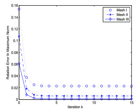
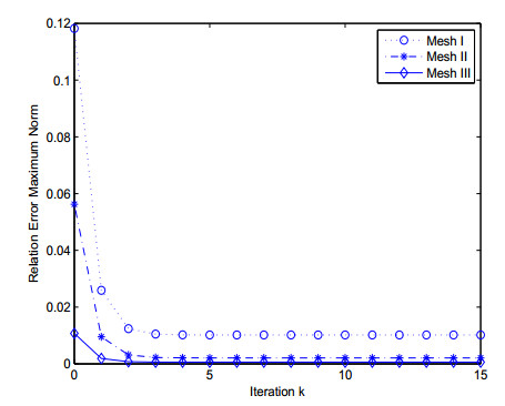
In this study, based on a general ellipsoidal artificial boundary, we present a Dirichlet-Neumann (D-N) alternating algorithm for exterior three dimensional (3-D) Poisson problem. By using the series concerning the ellipsoidal harmonic functions, the exact artificial boundary condition is derived. The convergence analysis and the error estimation are carried out for the proposed algorithm. Finally, some numerical examples are given to show the effectiveness of this method.
- D-N alternating algorithm,
- exterior 3-D poisson problem,
- ellipsoidal artificial boundary,
- natural boundary reduction
Citation: Xuqiong Luo. A D-N alternating algorithm for exterior 3-D problem with ellipsoidal artificial boundary[J]. AIMS Mathematics, 2022, 7(1): 455-466. doi: 10.3934/math.2022029

Related Papers:

Abstract

In this study, based on a general ellipsoidal artificial boundary, we present a Dirichlet-Neumann (D-N) alternating algorithm for exterior three dimensional (3-D) Poisson problem. By using the series concerning the ellipsoidal harmonic functions, the exact artificial boundary condition is derived. The convergence analysis and the error estimation are carried out for the proposed algorithm. Finally, some numerical examples are given to show the effectiveness of this method.

References

[1]	K. Bathe, E. L. Wilson, Numerical methods in finite element analysis, Englewood Cliffs: Prentice-Hall, 1976. doi: 10.1016/0898-1221(77)90079-7.
[2]	D. J. Evans, Numerical solution of exterior problems by the peripheral block over-relaxation method, IMA J. Appl. Math., 19 (1977), 399–405. doi: 10.1093/imamat/19.4.399. doi: 10.1093/imamat/19.4.399
[3]	C. A. Brebbia, Boundary element method in engineering, Berlin: Spring-Verlag, 1982.
[4]	D. Givoli, Numerical methods for problems in infinite domains, Amsterdam: Elsevier, 1992.
[5]	J. L. Zhu, Boundary element analysis for elliptic boundary value problems, Beijing: Science Press, 1992.
[6]	K. Feng, Finite element method and natural boundary reduction, In: Proceedings of the international congress of mathematicians, 1983, 1439–1453.
[7]	K. Feng, D. H. Yu, Canonical integral equations of elliptic boundary value problems and their numerical solutions, In: Proceedings of China-France symposium on the finite element method, Beijing: Science Press, 1983,211–252.
[8]	J. B. Keller, D. Givoli, Exact non-reflecting boundary conditions, J. Comput. Phys., 82 (1989), 172–192. doi: 10.1016/0021-9991(89)90041-7. doi: 10.1016/0021-9991(89)90041-7
[9]	H. D. Han, X. N. Wu, Approximation of infinite boundary condition and its application to finite element method, J. Comput. Math., 3 (1985), 179–192.
[10]	H. D. Han, X. N. Wu, The approximation of the exact boundary conditions at an artificial boundary for linear elastic equations and its applications, Math. Comput., 59 (1992), 21–37. doi: 10.1090/S0025-5718-1992-1134732-0. doi: 10.1090/S0025-5718-1992-1134732-0
[11]	D. Givoli, J. B. Keller, A finite element method for large domains, Comput. Methods Appl. M., 76 (1989), 41–66. doi: 10.1016/0045-7825(89)90140-0. doi: 10.1016/0045-7825(89)90140-0
[12]	M. J. Grote, J. B. Keller, On nonreflecting boundary conditions, J. Comput. Phys., 122 (1995), 231–243. doi: 10.1006/jcph.1995.1210. doi: 10.1006/jcph.1995.1210
[13]	D. Givoli, J. B. Keller, Special finite elements for use with high-order boundary conditions, Comput. Methods Appl. M., 119 (1994), 119–213. doi: 10.1016/0045-7825(94)90089-2. doi: 10.1016/0045-7825(94)90089-2
[14]	F. Brezzi, C. Johnson, On the coupling of boundary integral and finite element methods, Calcolo, 16 (1979), 189–201. doi: 10.1007/BF02575926. doi: 10.1007/BF02575926
[15]	C. Johnson, J. C. Nedelec, On the coupling of boundary integral and finite element methods, Math. Comp., 35 (1980), 1063–1079. doi: 10.1090/S0025-5718-1980-0583487-9. doi: 10.1090/S0025-5718-1980-0583487-9
[16]	D. H. Yu, Discretization of non-overlapping domain decomposition method for unbounded domains and its convergence (Chinese), Math. Numer. Sinica, 18 (1996), 328–336. doi: 10.12286/jssx.1996.3.328. doi: 10.12286/jssx.1996.3.328
[17]	D. H. Yu, Natural boundary integral mehtod and its applications, Dordrecht: Klumer Academic Publishers, 2002.
[18]	J. M. Wu, D. H. Yu, The natural integral equations of 3-D harmonic problems and their numerical solution (Chinese), Math. Numer. Sinica, 20 (1998), 419–430. doi: 10.12286/jssx.1998.4.419. doi: 10.12286/jssx.1998.4.419
[19]	J. M. Wu, D. H. Yu, The overlapping domain decomposition method for harmonic equation over exterior three-dimensional domain, J. Comput. Math., 18 (2000), 83–94.
[20]	H. Y. Huang, D. H. Yu, Natural boundary element method for three dimensional exterior harmonic problem with an inner prolate spheriod boundary, J. Comput. Math., 24 (2006), 193–208.
[21]	H. Y. Huang, D. J. Liu, D. H. Yu, Solution of exterior problem using ellipsoidal artificial boundary, J. Comput. Appl. Math., 231 (2009), 434–446. doi: 10.1016/j.cam.2009.03.009. doi: 10.1016/j.cam.2009.03.009
[22]	X. Q. Luo, Q. K. Du, H. Y. Huang, T. S. He, A Schwarz alternating algorithm for a three-dimensional exterior harmonic problem with prolate spheroid boundary, Comput. Math. Appl., 65 (2013), 1129–1139. doi: 10.1016/j.camwa.2013.02.004. doi: 10.1016/j.camwa.2013.02.004
[23]	X. Q. Luo, Q. K. Du, L. B. Liu, A D-N alternating algorithm for exterior 3-D poisson problem with prolate spheroid boundary, Appl. Math. Comput., 269 (2015), 252–264. doi: 10.1016/j.amc.2015.07.063. doi: 10.1016/j.amc.2015.07.063
[24]	C. S. Chen, A. Karageorghis, L. Amuzu, Kansa RBF collocation method with auxiliary boundary centres for high order BVPs, J. Comput. Appl. Math., 398 (2021), 113680. doi: 10.1016/j.cam.2021.113680. doi: 10.1016/j.cam.2021.113680
[25]	R. Cavoretto, A. De Rossi, An adaptive LOOCV-based refinement scheme for RBF collocation methods over irregular domains, Appl. Math. Lett., 103 (2020), 106178. doi: 10.1016/j.aml.2019.106178. doi: 10.1016/j.aml.2019.106178
[26]	R. Cavoretto, A. De Rossi, A two-stage adaptive scheme based on RBF collocation for solving elliptic PDEs, Comput. Math. Appl., 79 (2020), 3206–3222. doi: 10.1016/j.camwa.2020.01.018. doi: 10.1016/j.camwa.2020.01.018
[27]	E. W. Hobson, The theory of spherical and ellipsoidal harmonics (Bateman Manuscript Project), London: McGraw-Hill, 1955. doi: 10.2307/3607762.

Reader Comments

Your name:*

Email:*
© 2022 the Author(s), licensee AIMS Press. This is an open access article distributed under the terms of the Creative Commons Attribution License (http://creativecommons.org/licenses/by/4.0)