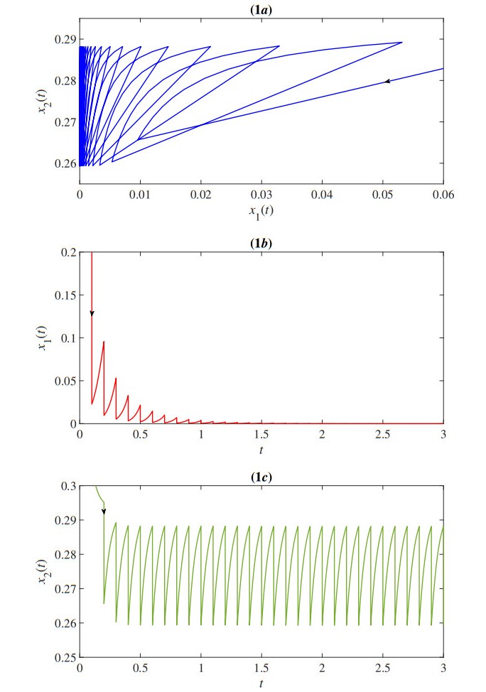
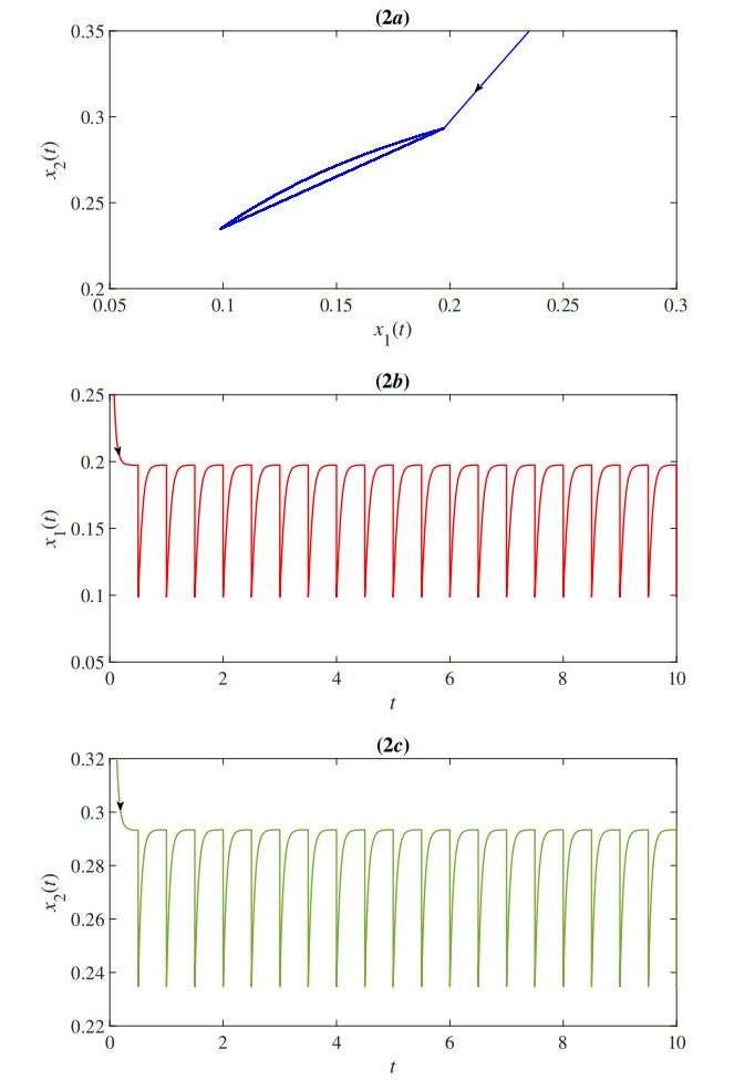
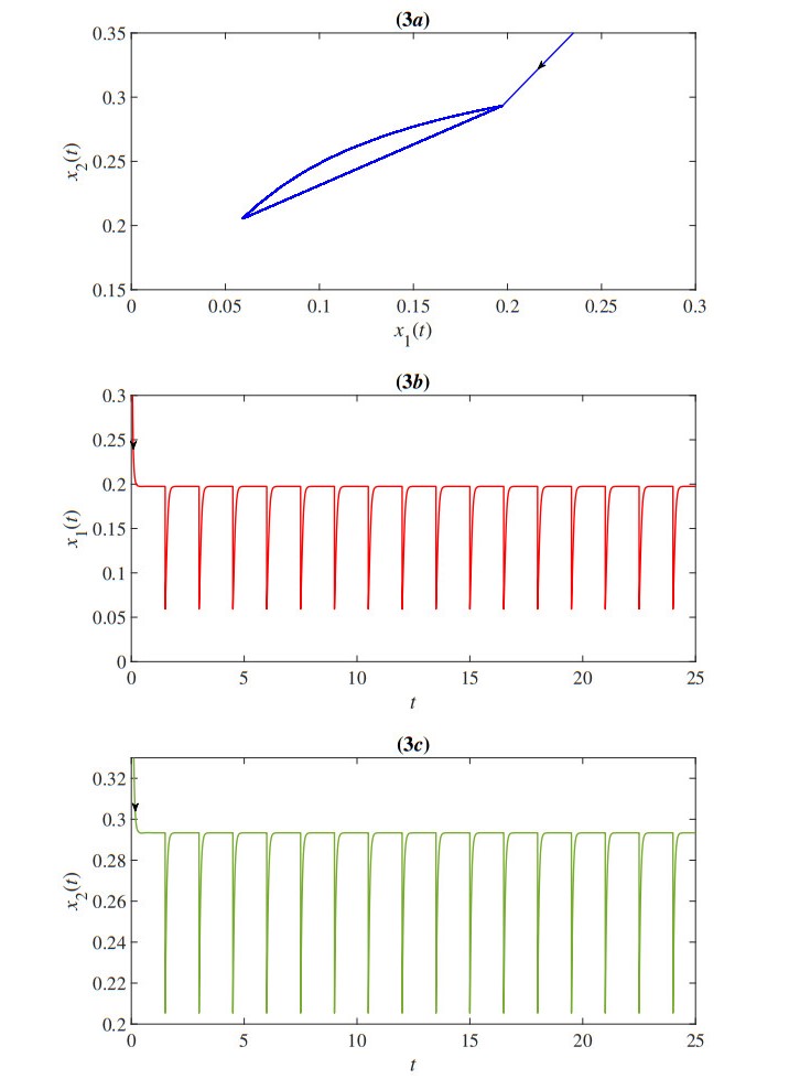
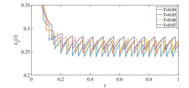
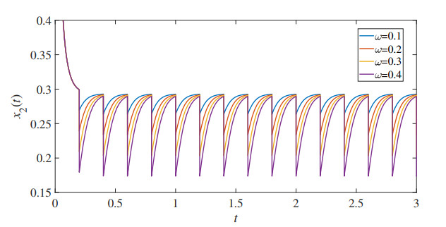
In this paper, we proposed a mathematical model of the population density of Indo-Pacific mackerel (Rastrelliger brachysoma) and the population density of small fishes based on the impulsive fishery. The model also considers the effects of the toxic environment that is the major problem in the water. The developed impulsive mathematical model was analyzed theoretically in terms of existence and uniqueness, positivity, and upper bound of the solution. The obtained solution has a periodic behavior that is suitable for the fishery. Moreover, the stability, permanence, and positive of the periodic solution are investigated. Then, we obtain the parameter conditions of the model for which Indo-Pacific mackerel conservation might be expected. Numerical results were also investigated to confirm our theoretical results. The results represent the periodic behavior of the population density of the Indo-Pacific mackerel and small fishes. The outcomes showed that the duration and quantity of fisheries were the keys to prevent the extinction of Indo-Pacific mackerel.
Citation: Din Prathumwan, Kamonchat Trachoo, Wasan Maiaugree, Inthira Chaiya. Preventing extinction in Rastrelliger brachysoma using an impulsive mathematical model[J]. AIMS Mathematics, 2022, 7(1): 1-24. doi: 10.3934/math.2022001
In this paper, we proposed a mathematical model of the population density of Indo-Pacific mackerel (Rastrelliger brachysoma) and the population density of small fishes based on the impulsive fishery. The model also considers the effects of the toxic environment that is the major problem in the water. The developed impulsive mathematical model was analyzed theoretically in terms of existence and uniqueness, positivity, and upper bound of the solution. The obtained solution has a periodic behavior that is suitable for the fishery. Moreover, the stability, permanence, and positive of the periodic solution are investigated. Then, we obtain the parameter conditions of the model for which Indo-Pacific mackerel conservation might be expected. Numerical results were also investigated to confirm our theoretical results. The results represent the periodic behavior of the population density of the Indo-Pacific mackerel and small fishes. The outcomes showed that the duration and quantity of fisheries were the keys to prevent the extinction of Indo-Pacific mackerel.

| [1] |
G. Ballinger, X. Liu, Permanence of population growth models with impulsive effects, Math. Comput. Model., 26 (1997), 59–72. doi: 10.1016/s0895-7177(97)00240-9. doi: 10.1016/s0895-7177(97)00240-9

|
| [2] |
E. Bergami, S. Pugnalini, M. Vannuccini, L. Manfra, C. Faleri, F. Savorelli, et al., Long-term toxicity of surface-charged polystyrene nanoplastics to marine planktonic species dunaliella tertiolecta and artemia franciscana, Aquat. Toxicol., 189 (2017), 159–169. doi: 10.1016/j.aquatox.2017.06.008. doi: 10.1016/j.aquatox.2017.06.008
|
| [3] |
G. Bueno, D. Bureau, J. Skipper-Horton, R. Roubach, F. Mattos, F. Bernal, Mathematical modeling for the management of the carrying capacity of aquaculture enterprises in lakes and reservoirs, Pesq. Agropec. Bras., 52 (2017), 695–706. doi: 10.1590/S0100-204X2017000900001. doi: 10.1590/S0100-204X2017000900001
|
| [4] |
B. R. Chavan, A. Yakupitiyage, S. Kumar, Mathematical modeling of drying characteristics of indian mackerel (Rastrilliger kangurta) in solar-biomass hybrid cabinet dryer, Dry. Technol., 26 (2018), 1552–1562. doi: 10.1080/07373930802466872. doi: 10.1080/07373930802466872
|
| [5] | B. Collette, C. Nauen, Fao species catalogue, Vol. 2: Scombrids of the world: An annotated and illustrated catalogue of tunas, mackerels, bonitos and related species known to date, Food and Agriculture Organization of the United Nations (FAO) Fisheries Synopsis, 1983. |
| [6] |
A. C. Dragon, I. Senina, N. T. Hintzen, P. Lehodey, Modelling south pacific jack mackerel spatial population dynamics and fisheries, Fish. Oceanogr., 27 (2018), 97–113. doi: 10.1111/fog.12234. doi: 10.1111/fog.12234
|
| [7] |
T. Hallam, R. Lassiter, S. Henson, Modeling fish population dynamics, Nonlinear Anal.: Theory Methods Appl., 40 (2000), 227–250. doi: 10.1016/s0362-546x(00)85013-0. doi: 10.1016/s0362-546x(00)85013-0
|
| [8] |
Y. Hashiguchi, M. R. Zakaria, T. Maeda, M. Z. M. Yusoff, M. A. Hassan, Y. Shirai, Toxicity identification and evaluation of palm oil mill effluent and its effects on the planktonic crustacean daphnia magna, Sci. Total Environ., 710 (2020), 136277. doi: 10.1016/j.scitotenv.2019.136277. doi: 10.1016/j.scitotenv.2019.136277
|
| [9] |
M. Hjorth, I. Dahllöf, V. E. Forbes, Effects on the function of three trophic levels in marine plankton communities under stress from the antifouling compound zinc pyrithione, Aquat. Toxicol., 77 (2006), 105–115. doi: 10.1016/j.aquatox.2005.11.003. doi: 10.1016/j.aquatox.2005.11.003
|
| [10] |
T. Jansen, H. Gislason, Population structure of Atlantic Mackerel (Scomber scombrus), PloS One, 8 (2018), e64744. doi: 10.1371/journal.pone.0064744. doi: 10.1371/journal.pone.0064744
|
| [11] |
R. Khatun, H. Biswas, Mathematical modeling applied to renewable fishery management, Math. Model. Eng. Probl., 6 (2019), 121–128. doi: 10.18280/mmep.060116. doi: 10.18280/mmep.060116
|
| [12] |
S. Kongseng, R. Phoonsawat, A. Swatdipong, Individual assignment and mixed-stock analysis of short mackerel (Rastrelliger brachysoma) in the inner and eastern gulf of Thailand: Contrast migratory behavior among the fishery stocks, Fish. Res., 221 (2020), 105372. doi: 10.1016/j.fishres.2019.105372. doi: 10.1016/j.fishres.2019.105372
|
| [13] | A. Lakmeche, O. Arini, Bifurcation of non-trivial periodic solutions of impulsive differential equations arising chemotherapeutic treatment, Dynam. Contin. Discrete Impuls., 7 (2000), 265–287. |
| [14] | V. Lakshmikantham, D. Bainov, P. Simeonov, Theory of impulsive differential equations, World Scientific, 1989. |
| [15] |
D. Liang, G. Y. Sun, W. Q. Wang, Second-order characteristic schemes in time and age for a nonlinear age-structured population model, J. Comput. Appl. Math., 235 (2011), 3841–3858. doi: 10.1016/j.cam.2011.01.031. doi: 10.1016/j.cam.2011.01.031
|
| [16] |
B. Liu, Y. Zhi, L. S. Chen, The dynamics of a predator-prey model with ivlev's functional response concerning integrated pest management, Acta Math. Applicatae Sin., 20 (2004), 133–146. doi: 10.1007/s10255-004-0156-0. doi: 10.1007/s10255-004-0156-0
|
| [17] |
N. Niamaimandi, F. Kaymaram, J. P. Hoolihan, G. H. Mohammadi, S. M. R. Fatemi, Population dynamics parameters of narrow-barred spanish mackerel, Scomberomorus commerson (lacèpéde, 1800), from commercial catch in the northern Persian Gulf, Glob. Ecol. Conserv., 4 (2015), 666–672. doi: 10.1016/j.gecco.2015.10.012. doi: 10.1016/j.gecco.2015.10.012
|
| [18] | Fisheries statistics of thailand 2018, Fisheries Development Policy and Planning Division, Department of Fisheries, Ministry of Agriculture and Cooperatives, 2020. Available from: https://www4.fisheries.go.th/local/file_document/20210520115148_new.pdf. |
| [19] |
R. P. Kaur, A. Sharma, A. K. Sharma, The impact of additional food on plankton dynamics in the absence andpresence of toxicity, Biosystems, 202 (2021), 104359. doi: 10.1016/j.biosystems.2021.104359. doi: 10.1016/j.biosystems.2021.104359
|
| [20] | D. Randall, T. Tsui, Ammonia toxicity in fish, Mar. Pollut. Bull., 45 (2002), 17–23. doi: 10.1016/s0025-326x(02)00227-8. |
| [21] |
C. Raymond, A. Hugo, M. Kungaro, Modeling dynamics of prey-predator fishery model with harvesting: A bioeconomic model, J. Appl. Math., 2019 (2019), 2601648. doi: 10.1155/2019/2601648. doi: 10.1155/2019/2601648
|
Figures(5) / Tables(1)

Din Prathumwan, Kamonchat Trachoo, Wasan Maiaugree, Inthira Chaiya. Preventing extinction in Rastrelliger brachysoma using an impulsive mathematical model[J]. AIMS Mathematics, 2022, 7(1): 1-24. doi: 10.3934/math.2022001


 DownLoad: