Analysis of 2D heat conduction in nonlinear functionally graded materials using a local semi-analytical meshless method

Chao Wang; Fajie Wang; Yanpeng Gong; Chao Wang; Fajie Wang; Yanpeng Gong

doi:10.3934/math.2021726

AIMS Mathematics

2021, Volume 6, Issue 11: 12599-12618. doi: 10.3934/math.2021726

Previous Article Next Article

Research article

Analysis of 2D heat conduction in nonlinear functionally graded materials using a local semi-analytical meshless method

Chao Wang ¹,
Fajie Wang ^{1,2
,
,},
Yanpeng Gong ^{3
,
,}

1.
College of Mechanical and Electrical Engineering, National Engineering Research Center for Intelligent Electrical Vehicle Power System, Qingdao University, Qingdao 266071, China
2.
Institute of Mechanics for Multifunctional Materials and Structures, Qingdao University, Qingdao 266071, China
3.
Institute of Electronics Packaging Technology and Reliability, Faculty of Materials and Manufacturing, Beijing University of Technology, Beijing 100124, China

Received: 05 July 2021 Accepted: 24 August 2021 Published: 01 September 2021
MSC : 65N35, 68W99, 80M22

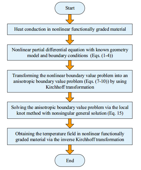
This paper proposes a local semi-analytical meshless method for simulating heat conduction in nonlinear functionally graded materials. The governing equation of heat conduction problem in nonlinear functionally graded material is first transformed to an anisotropic modified Helmholtz equation by using the Kirchhoff transformation. Then, the local knot method (LKM) is employed to approximate the solution of the transformed equation. After that, the solution of the original nonlinear equation can be obtained by the inverse Kirchhoff transformation. The LKM is a recently proposed meshless approach. As a local semi-analytical meshless approach, it uses the non-singular general solution as the basis function and has the merits of simplicity, high accuracy, and easy-to-program. Compared with the traditional boundary knot method, the present scheme avoids an ill-conditioned system of equations, and is more suitable for large-scale simulations associated with complicated structures. Three benchmark numerical examples are provided to confirm the accuracy and validity of the proposed approach.
- semi-analytical meshless method,
- local knot method,
- Kirchhoff transformation,
- nonlinear functionally graded material,
- heat conduction
Citation: Chao Wang, Fajie Wang, Yanpeng Gong. Analysis of 2D heat conduction in nonlinear functionally graded materials using a local semi-analytical meshless method[J]. AIMS Mathematics, 2021, 6(11): 12599-12618. doi: 10.3934/math.2021726

Related Papers:

Abstract

This paper proposes a local semi-analytical meshless method for simulating heat conduction in nonlinear functionally graded materials. The governing equation of heat conduction problem in nonlinear functionally graded material is first transformed to an anisotropic modified Helmholtz equation by using the Kirchhoff transformation. Then, the local knot method (LKM) is employed to approximate the solution of the transformed equation. After that, the solution of the original nonlinear equation can be obtained by the inverse Kirchhoff transformation. The LKM is a recently proposed meshless approach. As a local semi-analytical meshless approach, it uses the non-singular general solution as the basis function and has the merits of simplicity, high accuracy, and easy-to-program. Compared with the traditional boundary knot method, the present scheme avoids an ill-conditioned system of equations, and is more suitable for large-scale simulations associated with complicated structures. Three benchmark numerical examples are provided to confirm the accuracy and validity of the proposed approach.

References

[1]	L. L. Cao, Q. H. Qin, N. Zhao, Hybrid graded element model for transient heat conduction in functionally graded materials, Acta Mech. Sin., 28 (2012), 128-139. doi: 10.1007/s10409-011-0543-8
[2]	A. Lal, H. N. Singh, N. L. Shegokar, FEM model for stochastic mechanical and thermal postbuckling response of functionally graded material plates applied to panels with circular and square holes having material randomness, Int. J. Mech. Sci., 62 (2012), 18-33. doi: 10.1016/j.ijmecsci.2012.05.010
[3]	S. Akbarpour, H. R. Motamedian, A. Abedian, Micromechanical fem modeling of thermal stresses in functionally graded materials, In: ICAS Secretariat - 26th Congress of International Council of the Aeronautical Sciences 2008, ICAS 2008, 2008, 2851-2859.
[4]	Y. Chai, W. Li, Z. Liu, Analysis of transient wave propagation dynamics using the enriched finite element method with interpolation cover functions, Appl. Math. Comput., 412 (2022), 126564.
[5]	A. Sutradhar, G. H. Paulino, The simple boundary element method for transient heat conduction in functionally graded materials, Comput. Method. Appl. M., 193 (2004), 4511-4539. doi: 10.1016/j.cma.2004.02.018
[6]	M. I. Azis, D. L. Clements, Nonlinear transient heat conduction problems for a class of inhomogeneous anisotropic materials by BEM, Eng. Anal. Bound. Elem., 32 (2008), 1054-1060. doi: 10.1016/j.enganabound.2007.04.007
[7]	M. Tanaka, T. Matsumoto, Y. Suda, S. Takakuwa, A dual reciprocity time-stepping BEM applied to the transient heat conduction problem of functionally graded materials, Transactions of the Japan Society of Mechanical Engineers Series A, 68 (2002), 1702-1707. doi: 10.1299/kikaia.68.1702
[8]	B. L. Wang, Z. H. Tian, Application of finite element-finite difference method to the determination of transient temperature field in functionally graded materials, Finite Elem. Anal. Des., 41 (2005), 335-349. doi: 10.1016/j.finel.2004.07.001
[9]	C. Wang, Z. P. Qiu, Interval finite difference method for steady-state temperature field prediction with interval parameters, Acta Mech. Sin., 30 (2014), 161-166. doi: 10.1007/s10409-014-0020-2
[10]	C. Wang, Z. P. Qiu, Fuzzy finite difference method for heat conduction analysis with uncertain parameters, Acta Mech. Sin., 30 (2014), 383-390. doi: 10.1007/s10409-014-0036-7
[11]	W. Li, Q. Zhang, Q. Gui, Y. Chai, A coupled FE-meshfree triangular element for acoustic radiation problems, Int. J. Comput. Meth., 18 (2020), 2041002.
[12]	S. S. Saliba, L. Gori, R. L. Pitangueira, A coupled finite element-meshfree smoothed point interpolation method for nonlinear analysis, Eng. Anal. Bound. Elem., 128 (2021), 1-18. doi: 10.1016/j.enganabound.2021.03.015
[13]	V. Sladek, J. Sladek, M. Tanaka, C. Zhang, Transient heat conduction in anisotropic and functionally graded media by local integral equations, Eng. Anal. Bound. Elem., 29 (2005), 1047-1065. doi: 10.1016/j.enganabound.2005.05.011
[14]	J. Sladek, V. Sladek, C. Hellmich, J. Eberhardsteiner, Heat conduction analysis of 3-D axisymmetric and anisotropic FGM bodies by meshless local Petrov-Galerkin method, Comput. Mech., 39 (2007), 323-333.
[15]	A. R. Ahmad, A. Bagri, S. Bordas, T. Rabczuk, Analysis of thermoelastic waves in a two-dimensional functionally graded materials domain by the meshless local Petrov-Galerkin (MLPG) method, CMES-Computer Modeling in Engineering & Sciences, 65 (2010), 27-74.
[16]	Y. Wang, Y. Gu, J. Liu, A domain-decomposition generalized finite difference method for stress analysis in three-dimensional composite materials, Appl. Math. Lett., 104 (2020), 106226. doi: 10.1016/j.aml.2020.106226
[17]	W. Qu, H. He, A spatial-temporal GFDM with an additional condition for transient heat conduction analysis of FGMs, Appl. Math. Lett., 110 (2020), 106579. doi: 10.1016/j.aml.2020.106579
[18]	Q. Zhao, C. M. Fan, F. Wang, W. Qu, Topology optimization of steady-state heat conduction structures using meshless generalized finite difference method, Eng. Anal. Bound. Elem., 119 (2020), 13-24. doi: 10.1016/j.enganabound.2020.07.002
[19]	P. W. Li, Space-time generalized finite difference nonlinear model for solving unsteady Burgers' equations, Appl. Math. Lett., 114 (2021), 106896. doi: 10.1016/j.aml.2020.106896
[20]	F. Wang, W. Chen, C. Zhang, J. Lin, Analytical evaluation of the origin intensity factor of time-dependent diffusion fundamental solution for a matrix-free singular boundary method formulation, Appl. Math. Model., 49 (2017), 647-662. doi: 10.1016/j.apm.2017.02.044
[21]	Z. Fu, W. Chen, P. Wen, C. Zhang, Singular boundary method for wave propagation analysis in periodic structures, J. Sound Vib., 425 (2018), 170-188. doi: 10.1016/j.jsv.2018.04.005
[22]	X. Wei, W. Luo, 2.5D singular boundary method for acoustic wave propagation, Appl. Math. Lett., 112 (2021), 106760. doi: 10.1016/j.aml.2020.106760
[23]	L. Qiu, F. Wang, J. Lin, A meshless singular boundary method for transient heat conduction problems in layered materials, Comput. Math. Appl., 78 (2019), 3544-3562. doi: 10.1016/j.camwa.2019.05.027
[24]	F. Wang, W. Chen, Q. Hua, A simple empirical formula of origin intensity factor in singular boundary method for two-dimensional Hausdorff derivative Laplace equations with Dirichlet boundary, Comput. Math. Appl., 76 (2018), 1075-1084. doi: 10.1016/j.camwa.2018.05.041
[25]	Z. J. Fu, W. Chen, Q. H. Qin, Boundary knot method for heat conduction in nonlinear functionally graded material, Eng. Anal. Bound. Elem., 35 (2011), 729-734. doi: 10.1016/j.enganabound.2010.11.013
[26]	Z. J. Fu, J. H. Shi, W. Chen, L. W. Yang, Three-dimensional transient heat conduction analysis by boundary knot method, Math. Comput. Simulat., 165 (2019), 306-317. doi: 10.1016/j.matcom.2018.11.025
[27]	C. M. Fan, Y. K. Huang, P. W. Li, Y. T. Lee, Numerical solutions of two-dimensional stokes flows by the boundary knot method, CMES-Computer Modeling in Engineering and Sciences, 105 (2015), 491-515.
[28]	L. Sun, C. Zhang, Y. Yu, A boundary knot method for 3D time harmonic elastic wave problems, Appl. Math. Lett., 104 (2020), 106210. doi: 10.1016/j.aml.2020.106210
[29]	H. Wang, Q. H. Qin, Y. L. Kang, A meshless model for transient heat conduction in functionally graded materials, Comput. Mech., 38 (2006), 51-60. doi: 10.1007/s00466-005-0720-3
[30]	L. Marin, D. Lesnic, The method of fundamental solutions for nonlinear functionally graded materials, Int. J. Solids Struct., 44 (2007), 6878-6890. doi: 10.1016/j.ijsolstr.2007.03.014
[31]	G. Fairweather, A. Karageorghis, The method of fundamental solutions for elliptic boundary value problems, Adv. Comput. Math., 9 (1998), 69-95. doi: 10.1023/A:1018981221740
[32]	F. Wang, C. S. Liu, W. Qu, Optimal sources in the MFS by minimizing a new merit function: Energy gap functional, Appl. Math. Lett., 86 (2018), 229-235. doi: 10.1016/j.aml.2018.07.002
[33]	C. M. Fan, Y. K. Huang, C. S. Chen, S. R. Kuo, Localized method of fundamental solutions for solving two-dimensional Laplace and biharmonic equations, Eng. Anal. Bound. Elem., 101 (2019), 188-197. doi: 10.1016/j.enganabound.2018.11.008
[34]	F. Wang, Y. Gu, W. Qu, C. Zhang, Localized boundary knot method and its application to large-scale acoustic problems, Comput. Method. Appl. M., 361 (2020), 112729. doi: 10.1016/j.cma.2019.112729
[35]	X. Yue, F. Wang, C. Zhang, H. Zhang, Localized boundary knot method for 3D inhomogeneous acoustic problems with complicated geometry, Appl. Math. Model., 92 (2021), 410-421. doi: 10.1016/j.apm.2020.11.022
[36]	W. Qu, C. M. Fan, Y. Gu, F. Wang, Analysis of three-dimensional interior acoustic fields by using the localized method of fundamental solutions, Appl. Math. Model., 76 (2019), 122-132. doi: 10.1016/j.apm.2019.06.014
[37]	Y. Gu, C. M. Fan, R. P. Xu, Localized method of fundamental solutions for large-scale modeling of two-dimensional elasticity problems, Appl. Math. Lett., 93 (2019), 8-14. doi: 10.1016/j.aml.2019.01.035
[38]	F. Wang, C. M. Fan, Q. Hua, Y. Gu, Localized MFS for the inverse Cauchy problems of two-dimensional Laplace and biharmonic equations, Appl. Math. Comput., 364 (2020), 124658.
[39]	X. Li, S. Li, On the augmented moving least squares approximation and the localized method of fundamental solutions for anisotropic heat conduction problems, Eng. Anal. Bound. Elem., 119 (2020), 74-82. doi: 10.1016/j.enganabound.2020.07.007
[40]	Y. Gu, C. M. Fan, W. Qu, F. Wang, Localized method of fundamental solutions for large-scale modelling of three-dimensional anisotropic heat conduction problems - Theory and MATLAB code, Comput. Struct., 220 (2019), 144-155. doi: 10.1016/j.compstruc.2019.04.010
[41]	F. Wang, C. M. Fan, C. Zhang, J. Lin, A localized space-time method of fundamental solutions for diffusion and convection-diffusion problems, Adv. Appl. Math. Mech., 12 (2020), 940-958. doi: 10.4208/aamm.OA-2019-0269
[42]	W. Qu, C. M. Fan, X. Li, Analysis of an augmented moving least squares approximation and the associated localized method of fundamental solutions, Comput. Math. Appl., 80 (2020), 13-30. doi: 10.1016/j.camwa.2020.02.015
[43]	W. Li, Localized method of fundamental solutions for 2D harmonic elastic wave problems, Appl. Math. Lett., 112 (2021), 106759. doi: 10.1016/j.aml.2020.106759
[44]	X. Li, S. Li, A linearized element-free Galerkin method for the complex Ginzburg-Landau equation, Comput. Math. Appl., 90 (2021), 135-147. doi: 10.1016/j.camwa.2021.03.027
[45]	X. Li, H. Dong, An element-free Galerkin method for the obstacle problem, Appl. Math. Lett., 112 (2021), 106724. doi: 10.1016/j.aml.2020.106724
[46]	X. Li, S. Li, A fast element-free Galerkin method for the fractional diffusion-wave equation, Appl. Math. Lett., 122 (2021), 107529. doi: 10.1016/j.aml.2021.107529
[47]	F. Wang, C. Wang, Z. Chen, Local knot method for 2D and 3D convection-diffusion-reaction equations in arbitrary domains, Appl. Math. Lett., 105 (2020), 106308. doi: 10.1016/j.aml.2020.106308
[48]	X. Yue, F. Wang, P. W. Li, C. M. Fan, Local non-singular knot method for large-scale computation of acoustic problems in complicated geometries, Comput. Math. Appl., 84 (2021), 128-143. doi: 10.1016/j.camwa.2020.12.014
[49]	W. Chen, M. Tanaka, A meshless, integration-free, and boundary-only RBF technique, Comput. Math. Appl., 43 (2002), 379-391. doi: 10.1016/S0898-1221(01)00293-0
[50]	J. Sladek, V. Sladek, Y. C. Hon, Inverse heat conduction problems by meshless local Petrov-Galerkin method, Eng. Anal. Bound. Elem., 30 (2006), 650-661. doi: 10.1016/j.enganabound.2006.03.003

Reader Comments

Your name:*

Email:*
© 2021 the Author(s), licensee AIMS Press. This is an open access article distributed under the terms of the Creative Commons Attribution License (http://creativecommons.org/licenses/by/4.0)