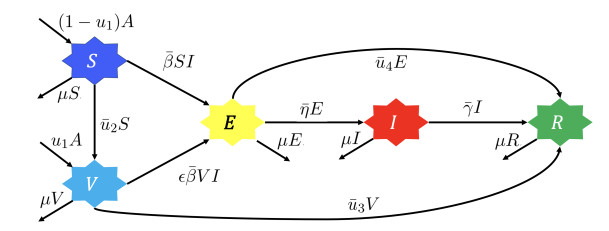
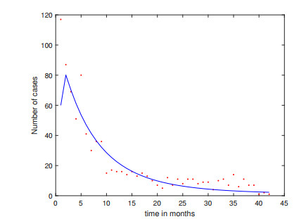
1.
Introduction
Measles is an infectious disease which was first acknowledged in Boston in 1657. Before the measles vaccine was released in 1954, the world experienced more than 135 million cases every year [1]. Measles is a highly contagious disease [2], in which humans were considered to be the main reservoir of the measles virus (paramyxovirus family) [3]. The virus can be transmitted through the air via respiratory secretions or aerosol droplets when an infected individuals sneezes or coughs, where the respiratory tract is the first organ in the human body to be affacted [1,2]. The measles virus can live in a room for up to two hours [4,5].
Measles does not have a special antiviral treatment [2]. Therefore, focusing on prevention, supportive care, and treatment of complications and secondary infections are the best management strategies for these cases [1]. Severe complications can be minimized through supportive care that ensures good nutrition, adequate fluid intake, and dehydration treatment with the recommended WHO oral rehydration solution. The concentration of vitamin A in children with severe measles is low, so providing this vitamin A can reduce morbidity and mortality. Vitamin A can increase the antibody response to the measles virus and reduce complications of measles [6]. WHO recommends that all children diagnosed with measles must receive two doses of vitamin A supplements given 24 hours apart [1,2]. Vitamin A for treatment of measles is administered once daily for two days [7]. In addition, vitamin A supplements have been shown to reduce the number of measles deaths [1,2]. A measles-containing vaccine can prevent measles [8]. The vaccines currently available are safe and effective and can be used interchangeably in the immunization program [9]. Mass immunization campaigns with routine measles vaccination for children in countries with high rates of cases and deaths are the leading public health strategies to reduce measles death globally [2]. There are two doses of the measles vaccine. The first dose should be given at the age of 12–15 months, while the second dose is usually given at the age of 4–6 years. However, the second dose can be given earlier, provided there is an interval time of at least 28 days from the first dose [10]. Accelerated immunization has a significant impact on reducing deaths due to measles. Some vaccines are almost 100% effective, e.g., two doses of MMR (Measles, Mumps, and Rubella) vaccine will protect 99% of people from measles.
Although immunization activities have been carried out, there were still many countries experiencing measles outbreaks in 2019. The WHO reported 413,308 measles cases through official monthly reports from 187 member states [11]. This situation has prevented the Health Assembly from eliminating measles in four WHO regions by 2015 and five regions by 2020. In 2017, Indonesia also experienced an increase in the number of individuals infected with measles [12]. Therefore, in implementing global targets to eliminate and control measles and rubella by 2020, hospitals are instructed to identify measles susceptible individuals by considering the mapping of cases and immunization status at the rural level [13].
Many authors have used mathematical models to understand the spread of measles. For example, a simple SEIR model was introduced by authors in [14] to understand the dynamics of measles when no interventions are included in the model. The authors in [15] discuss a relationship between mass vaccination and herd immunity in their research, while authors in [16] consider the impact of vaccine and death due to measles in their model. Authors in [17] discussed the transmission of measles in China by considering the seasonality spreading factor. Furthermore, authors in [18] consider early tests and therapy on the exposed individuals to avoid the further outbreak of measles. Unlike the aforementioned references, authors in [19] include passive immune groups in their model to analyze the impact of this group in the measles eradication strategy. Effect of quarantine compartment discussed by the authors in [20]. Furthermore, they find that quarantine intervention can help the success of a vaccination strategy to reduce the endemic level of measles in the population. Authors in [21] consider a vaccination model on measles transmission, where they found a possibility that the basic reproduction number less than one does not guarantee the disappearance of measles in the community due to the appearance of backward bifurcation phenomena. Some mathematical models for measles transmission using fractional derivatives were recently introduced [22,23,24,25]. All of these references state that immunization intervention could help to reduce the spread of measles. However, the high intensity of vaccination level comes with a high cost for intervention. Hence, an optimal means of intervention should be found.
Many researchers have long used the optimal control theory approach to find the most optimal solution in reducing disease spread, in this case, by using a time-dependent intervention in their model. Please see [26,27,28,29,30] for further references. Some researchers have implemented optimal control in their research on the measles transmission model [31,32,33]. However, all the studies previously mentioned on measles transmission did not include an analysis of cost-effectiveness in considering the interventions given. Cost-effectiveness analysis is a common analysis to determine the best strategy among different scenarios by considering its relative cost or the effect (in our case, reducing the number of infected individuals). Please see [26,34] for some references on the cost-effectiveness analysis in some epidemiological problems.
Based on the mentioned introduction, this article aims to determine the effectiveness of newborn and adult vaccination (first and second dose) and an early treatment to suppress the spread of measles in Jakarta, Indonesia. To achieve this aim, we construct an optimal control problem model that arises from a measles transmission model by considering four time-dependent control variables: The first dose of vaccine (newborn and adult population), the second dose of vaccine, and measles therapy. The model was constructed using a non-linear system of an ordinary differential equation. Although our model uses the same approach as several mentioned references (using the ODE model), our model considers more detailed types of vaccines, namely vaccinations for children and adults and the first and second stage of vaccinations. In addition, early detection of the latent phase was also included in the model. Furthermore, our paper uses incident data for the city of Jakarta, which has not been widely used, especially for its application to the optimal control problem, to determine the best possible strategies for measles eradication. Mathematical analysis was conducted regarding the positiveness of the solution, the basic reproduction number, existence and local stability criteria of all equilibrium points, and bifurcation analysis. Incidence data of measles in Jakarta was used to determine the best-fit parameters for our model. We detect the most significant parameters to determine the size of the basic reproduction using sensitivity analysis. Optimal control simulation is followed by cost-effectiveness analysis conducted for several possible scenarios to find the best strategies for the measles eradication program.
This article is presented as follows: We describe the model formulation in section 2. Section 3 analyzes the existence and stability of equilibrium points from the model, estimates infection rate and medical treatment rate parameters, and analyzes the sensitivity of basic reproduction number results together with bifurcation analysis. In section 4, we present our optimal control problem and numerically simulate it. We analyze the cost-effectiveness of our optimal control scenario in section 5. Finally, some conclusions are given in section 6.
2.
Model formulation
Measles is an infectious disease that spreads through direct contact or the air. After an individual is exposed to the measles virus, there is an incubation period before it can be transmitted to others. Those that are infected have lifelong immunity after recovering from measles. On the other hand, the measles vaccine has been used to prevent measles for many years. Most people who have not received the MMR vaccine will suffer from measles if they are exposed to the measles virus [2,4,9].
This paper aims to understand the impact of various strategies on the measles eradication program, namely newborn and adults vaccination, second dose vaccination, and medical treatment. To achieve this aim, let us consider that the human population at time t is divided into five subclasses: Susceptible (S(t)), vaccinated (V(t)), exposed (E(t)), infectious (I(t)), and recovered (R(t)). Hence the total of the human population denoted by N(t) is given by
For simplification, we use S,V,E,I,R instead of S(t),V(t),E(t),I(t),R(t), respectively. Description for each variable is given in Table 1. To construct the model, we use the transmission diagram in Figure 1 to depict the population, which describes our proposed model's transmission and transition processes.
Please note that u1 and ˉu2 are the first doses of vaccination, while ˉu3 is the second dose of vaccination given only to individuals who already have had their first vaccination (individual in V). In our model, the first dose of vaccination does not perfectly protect people from measles. However, this first dose could reduce the probability of successful infection in the amount of ϵ. If ϵ=0, then the first dose of vaccine protects people from measles perfectly, and vice versa for ϵ=1.
Community awareness of maintaining personal and family health can help reduce measles transmission. When individuals are exposed to the virus, they can obtain medical treatment, such as testing and measles therapy. This model includes the medical treatment intervention that will cure exposed individuals (E) at the rate of ˉu4 and transfer individuals from the E compartment to the recovered/immune (R) compartment. Furthermore, when susceptible (S) and vaccinated (V) individuals are infected due to direct contact with the infected compartment (I), they will be transferred into the exposed (E) compartment in which the symptoms of measles start to appear, such as high fever, a runny nose, a cough, red and watery eyes, and small white spots inside the cheeks [2]. After the incubation period (1ˉη), individuals in E will move to the I compartment, except for individuals who received measles therapy (ˉu4E), until the infected individuals are recovered at the rate of ˉγ and transferred to the R compartment. Each compartment will decrease in size due to natural death at a rate of μ. In this paper, we ignore the death rate induced by measles.
Based on the above assumptions and transmission diagram in Figure 1, our model read as follows:
where all parameters are positive. This system of equation is supplied with non-negative initial conditions: S>0,V≥0,E≥0,I≥0,R≥0. All parameters in the model are stated in Table 2. With our proposed model in (2.1), we can determine the best type of intervention between vaccination stages one and two, newborn or adult vaccination strategy, and the effect of early detection on measles infection through sensitivity analysis of the basic reproduction number of the model.
Before we analyze the model (2.1) regarding the existence and local stability criteria of the equilibrium point and how the basic reproduction number is related to it, we give some preliminary analysis of the model. We know that
and we assume that the number of natural deaths and newborns are equal and that there are no deaths related to measles, so we have dNdt=0, which implies that N(t)=N is a constant. Next, we will prove that the solution of system (2.1) for all t>0 will always be non-negative whenever the initial condition is non-negative. This result is stated in the following theorem.
Theorem 1. The solution of the model in system (2.1) with non-negative initial conditions will remain non-negative for all time t≥0.
Proof. Please see Appendix A.
According to the above analysis, we can conclude that our model is biologically well defined since the solution is always non-negative. Furthermore, since N(t) is always constant, and each variable in model (2.1) is always positive, then we know that each variable must be bounded. This result is stated in the following corollary.
Corollary 1. All variables in model (2.1) are bounded in visible domain defined by
3.
Model analysis
To simplify our model, we use the normalized quantities of each variable on our model instead of the actual population size. Since we know the total population is constant, let x1=SN,x2=VN,x3=EN,x4=IN,x5=RN. Since ∑5i=1xi=1, therefore x5=1−∑4i=1xi. Using the above scaling and also μ=AN, β=ˉβNμ, η=ˉημ, γ=ˉγμ, u2=ˉu2μ, u3=ˉu3μ, u4=ˉu4μ, and τ=μt, the scaled system of Eq (2.1) becomes
Henceforth, we analyze the above equation system to understand the qualitative behaviour of our proposed model in system (2.1).
3.1. Stability of the measles-free equilibrium (MFE) and the basic reproduction number
The measles model in system (3.1) has a unique trivial equilibrium, namely Ω1, which is given by
Some discussions regarding this equilibrium are given as follows:
Ratio of x2 and x1. It is essential to determine this ratio, which will indicate the success of the vaccination strategy by moving the susceptible proportion (x1) into the vaccinated proportion (x2). A larger ratio of x2x1 in Ω1 indicates that it is easier to control measles since vaccinated individuals have a smaller infection probability. From the ratio of x2 and x1 in the measles-free equilibrium, we have
Since ∂x†2x†1∂u1=1+u2(u3+1)(1−u1)2>0, then increasing the first dose of newborn vaccination intervention u1 will increase this ratio. Also, since ∂x†2x†1∂u2=1(u3+1)(1−u1)>0, increasing the first dose of adult vaccination u2 will also increase this ratio. On the other hand, because ∂x†2x†1∂u3=−(u1+u2)(u3+1)2(1−u1)<0, then enlarging u3 will reduce this ratio. This result does not show a contrapositive phenomenon, since more people enter x5 (recovered proportion) due to u3, which indicates a fully immune individual.
These results imply that increasing the proportion of newborns or susceptible individuals who receive a first dose of vaccination will increase the proportion of vaccinated individuals. The cause is that susceptible individuals who are given the first dose vaccine will then turn into vaccinated individuals. Also, if the rate of the second dose of vaccination increases, the vaccinated proportion will decrease because the vaccinated individuals with the second dose of vaccine will move to the recovered proportion.
Ratio of x5 and x2. It is important to consider this ratio that shows the success of measles awareness and vaccination strategy to move the vaccinated proportion (x2) into the recovered proportion (x5). Please note that x†5=u3(u1+u2)(1+u2)(1+u3). A larger value of x5x2 in Ω1 is better for controlling measles, since recovered individuals cannot be infected. Following the ratio of x5 and x2 in the measles-free equilibrium,
Since ∂x†5x†2∂u3=1>0, then increasing u3 also increases this ratio. Enlarging u3 means more people go to x5, which indicates fully immune individuals. This means it is suitable for the model, and the transition from x2 to x5 is only caused by the second dose of vaccine given. Furthermore, the displacement from vaccinated individuals to recovered individuals is not influenced by the first dose of vaccine.
Basic reproduction number. In many mathematical models, such as in [39,40,41,42,43], the basic reproduction number determines the behavior of their epidemiological model. We use the next generation matrix approach, which has been described in [44], to derive the basic reproduction number of our non-dimensionalized model (3.1). The transition matrix (Σ) and the transmission matrix (T) of system (3.1) are given by
Since the transmission matrix has a zero row, the next generation matrix is given by K=−ET∗TΣ−1E∗, where E∗ is an auxiliary matrix [10]T. Therefore, the basic reproduction of our proposed model is given as follows:
where ρ is the spectral radius operator. Having the basic reproduction number in hand, we give the local stability criteria of Ω1 in the following theorem.
Theorem 2. The measles-free equilibrium, Ω1, is locally asymptotically stable if R0<1.
Proof. Please see Appendix B for the proof.
As seen in Eq (3.6), the basic reproduction number is linear with respect to the infection parameter (β). This result means that the easier it is for measles to be transmitted, the more difficult it is for measles to disappear from the population. Therefore, it is necessary to reduce the size of the infection rate to reduce the amount of R0. It can be seen that because the vaccine efficacy (ϵ) is linear with respect to R0, the better the quality of the vaccine (the smaller value of ϵ) will increase the chances of the emergence of measles-free conditions. Furthermore, it is seen that the rate of early treatment is inversely proportional to R0. Therefore, it can be concluded that giving a treatment can increase the chance of eliminating measles in the field. Compared to all these results, the next question is: Which intervention should be prioritized if there are limited costs for interventions in the field? This will then be discussed in the chapter on optimal control.
3.2. Existence of the endemic equilibrium
The next equilibrium is the non-trivial equilibrium which describes a condition where measles persists in the population. We find that this equilibrium is unique if and only if the basic reproduction number is larger than unity. This result is stated in the following theorem.
Theorem 3. Model (3.1) has an endemic equilibrium point Ω2=(x‡1,x‡2,x‡3,x‡4) with
where x‡4 is the positive root of the following polynomial
if R0>1. Furthermore, there is no endemic equilibrium if R0<1.
Proof. Please see Appendix C for the proof.
3.3. Bifurcation analysis
In this section, we analyze the type of bifurcation of our non dimensional model in (3.1) using the well-known Castillo-Song bifurcation theorem [45]. The result is stated in the following theorem.
Theorem 4. The unique endemic equilibrium Ω2 of system (3.1) is locally asymptotically stable for R0>1 but close to 1.
Proof. Please see Appendix D for the proof.
The result in Theorem 4 states that our model always reaches a measles-free state whenever the basic reproduction number is smaller than one. When the basic reproduction number is equal to one, a change of stability occurs, where the measles-free equilibrium becomes unstable, and the non-trivial/endemic equilibrium arises and stable. The larger value of the basic reproduction number will increase the infected individuals' equilibrium state in the equilibrium point. The existence of forward bifurcation on our model indicates that the basic reproduction number becomes the only indicator for the disappearance of measles. As long as we can achieve a condition of R0<1, then measles will always disappear from the population.
3.4. Estimate the infection and medical treatment rate
In this paper, we used monthly measles data in Jakarta to estimate the infection and medical treatment rate parameters (β and u4). The data is a record of measles case numbers in Jakarta from January 2017 to June 2020. The aim is to find the best fit parameters β and u4 such that our model (2.1) fits the data. This aims to minimize the sum of square errors of
where Yj and I(tj) are the incidence data and the simulation result at time step j, respectively. We used nonlinear least square method to solve this problem numerically. We used the initial value (S0,V0,E0,I0,R0)=(444422,888844,80,60,9134223), while all parameter values are listed in Table 2. We used pre-estimated β=1.2527×10⁻⁹ (see [17]) and u4=0.25. Using the least square method, we obtained the best fit parameters of β=0.00000302513594,u4=0.312069708617258 and the visualization of the result is shown in Figure 2. The blue curve represents the simulation result of I(t) from model (2.1), while the red dot is Jakarta's monthly measles data from January 2017 to June 2020.
With those parameters, we obtained the value of the basic reproduction number of measles in Jakarta which is 2.22. This result implies that without any further improvement on measles eradication strategy, measles will be endemic in Jakarta. In Figure 2, we can see that the fitting result goes to 0. This is due to the short time of the simulation. However, if we carry out the simulation for a long time period, we can see that I(t) goes to 1796 (endemic equilibrium), which can be seen in Figure 3. Based on [3], measles Routine Immunization Coverage has decreased in Indonesia between 2012 and 2018. In the Jakarta area, measles vaccine coverage is still quite adequate when compared to the average measles coverage in Indonesia. There are still many measles cases in the Jakarta area and although various forms of intervention have been carried out, it shows that the efforts made have not been optimal in their implementation.
3.5. Analysis of the basic reproduction number
It is essential to understand how robust our model concerns the change of parameters in the basic reproduction number expression. Hence, we conducted a sensitivity analysis of the basic reproduction number to see the effect of the parameter uncertainty and sensitivity on any changes in the model parameter values. This result is important to consider how the basic reproduction number can affect the equilibrium points' existence and stability regarding the previous theorems. In this section, we will use model (2.1) again instead of the non-dimensionalized model to get a direct interpretation of our results. Hence, by substituting all non-dimensionalized parameters to their dimensionalized form, the basic reproduction number of model (2.1) is given as follows:
Please note that we neglect the "bar" sign for the sake of written simplification. We use elasticity ~R0 with respect to p which is the percentage change in ~R0 with respect to the percentage change in the p parameter [46] as follows:
All calculated results from elasticity of ~R0 with respect to all parameters are presented in Appendix E. Using the following parameter values μ=172.67×12,u1=0.85,u2=0.8572.67×12,u3=0.5272.67×12, u4=0.312069708617258, ϵ=0.07,γ=1.579, η=3011,β=0.00000302513594, A=1046762972.67×12 where ~R0=2.22, we calculated the elasticity of ~R0, which is given in Table 3. Based on the results of the sensitivity analysis in Table 3, it can be seen that the vaccination intervention in newborns is the most sensitive parameter on to change R0 significantly, followed by the first dose of vaccination in adults, the second dose of vaccination, and the rate of early treatment. Although the first dose of vaccine is considered the most influential, other forms of intervention still need to be implemented to achieve measles-free conditions more quickly. In addition, treatment is still needed so that the possibility of secondary infection in healthy people can be reduced.
We can see the elasticity of ~R0 on all parameters in Figure 4, where the X-axis is the elasticity value of a parameter and the Y-axis is the parameter. The interpretation of the elasticity εp~R0 is if εp~R0>0, and then every 1% increase in p parameter value causes an increase in the ~R0 value by εp~R0%. If εpR0<0, then every 1% increase in the value of the p parameter causes a decrease in the value of ~R0 by εp~R0%. For example, we interpreted εu1~R0 where the value of elasticity from u1 is -3.55. From prior data, we obtained ~R0=2.218 where u1=0.85 if we increase 1% of u1 by
In this situation, uold1=0.85 so unew1=0.8585, and we obtain ~R0=2.139 where other parameters except u1 are the same as the data that we use before. Note the value of εu1~R0=−3.55<0; this is the same as the previous one, meaning that when the value of u1 increases by 1%, the value of ~R0 will decrease as follows:
Other parameters can be interpreted in the same way. From Figure 4, we see u1 could suppress the value of ~R0 most significantly compared to other controls.
3.6. Sensitivity analysis of the first dose vaccination
We conducted the special case of sensitivity analysis in order to see how the first dose vaccination affects the size of ~R0 in this subsection. By setting u2=u3=u4 equal to zero and keeping the other parameters the same as before, solving ~R0 equal to one with respect to u∗1 gave us
We found u∗1=1.02. This value presented the critical level when the newborn first dose vaccination is the only strategy used in the field. Since εu1~R0<0, whenever u1 is chosen to be larger than 1.02, then measles can be eradicated from the population since the ~R0 is smaller than unity. To understand the dependency of ~R0 with respect to the first dose vaccination strategy, we provide the contour plot of ~R0 with respect to u1 and u2 in Figure 5. It is easy to see that increasing values of u1 and u2 partially can significantly reduce ~R0 non-linearly.
To analyze the dynamics of our proposed model (2.1) with respect to the change of both u1 and u2, we perform the trajectories of I(t) in Figure 6 by using the Runge-Kutta numerical scheme in Matlab. Our results indicate how the first dose vaccine succeeds in reducing the number of infected individuals. The first dose vaccine's effect does not appear early in the simulation since the dynamics of I still tend to the outbreak during this period of time. However, after the outbreak passes, the effect of the vaccine starts to take hold when the difference of I for different values of u1 and u2 becomes significantly different.
Based on the previous elasticity of ~R0, we know that u1 greatly affects the value of ~R0, while u2 has less elasticity. This can also be seen in Figure 6. Looking at Figure 6(a), (b), with an increase of 50 % of u2, the change in the infected individuals is not too great, and the change in the value of u1 simply affects the number of infected individuals. Meanwhile, in Figure 6, giving u1 is enough to dominate, so that changes in u2 do not show any significant changes.
4.
Optimal control problem
Based on the previous analysis of the basic reproduction number's sensitivity, we found that the first and second doses of vaccination and medical treatment can reduce the spread of measles. Increasing all of the mentioned forms of intervention is better for the measles eradication program. However, any intense intervention will come at a high cost of implementation. Hence, we have to find the optimal strategy to conduct these interventions. The question is, which means of intervention is a more reasonable choice based on their cost of intervention? Also, when do we have to give such high-intensity intervention? Finally, which combination of means of intervention should be chosen to provide the best result for the measles eradication strategy? To answer these questions, we modify our previous model in system (2.1) as an optimal control problem by treating the first and second doses of vaccination and medical treatment interventions as time-dependent variables.
4.1. Characterization of the optimal control problem
As mentioned before, we treat all means of intervention as time-dependent variables. Hence, we have:
Based on the above assumption, our proposed model in system (2.1) now reads as:
Please note that we may neglect R in the calculation of the optimal control problem to the fact that the population was assumed to be constant. Hence, we have R(t)=N(t)−S(t)−V(t)−E(t)−I(t).
Our optimal control problem aims to minimize the number of infected individuals with minimal intervention costs. Therefore, we define our cost function as follows:
where ω0,ω1,ω2,ω3, and ω4 are the positive weight parameters that will guarantee the balance of each component in the objective function. The first component in (4.2), i.e ω0I presents the cost related to the high number of infected individuals in the field such as cost of media campaign, economic cost, etc. The last four components in (4.2) present the cost of newborn vaccination, first dose adult vaccination, second dose vaccination, and medical treatment, respectively.
Let us define the following Hamiltonian of our problem:
Taking the derivative of H with respect to each state variable, the adjoint system is given by
Please note that system (4.4) was completed with a transversality condition zi(T)=0 for i=1,2,3,4. Furthermore, the optimality condition was taken by solving ∂H∂ui=0 with respect to each ui for i=1,2,3,4. Hence, we have
Taking the lower and upper bounds of our control variables as umini and umaxi, respectively, we have the optimal intervention as given by
4.2. Numerical experiment
To conduct the simulations in this section, we choose ω0=1,ω1=5,ω2=10,ω3=15, and ω4=30 to balance each term in the cost function (4.2). The optimality system which consisting set of equation for state (4.1), adjoint (4.4), and optimality condition (4.6) is solved using backward-forward sweep method which described in [47]. More examples on this method can be seen in [26,28] and references therein. The initial condition for state variable are taken as S(0)=444422,V(0)=888844,E(0)=80,I(0)=60. We conduct seven type of scenarios for our optimal control simulation based on which forms of intervention were used in the scenario (see Table 4). Each scenario was conducted for a short (T=months)andlong( T = 60 $ months) term simulations.
Please note that we conduct the results of each scenario on a figure in the following simulation results. The first row for each figure presents the comparison of the trajectory between infected individuals I(t) without (blue curve) and with (red curve) interventions implemented. The second row on each figure presents the dynamics of each control.
4.2.1. Strategy A (S–A)
For the first scenario, we conduct the simulation using all of the interventions to control the spread of measles. The simulation results using all interventions are given in Figure 7 for a short period of simulation and Figure 8 for a long period of simulation.
Note that in Figure 7, the number of infected individuals with control use increased at the start, but maximizing the number of vaccines and medical treatment quickly reduced the number of individuals infected. Even though the number of infected individuals can decrease quickly, a measles vaccine is still given, so each individual retains good immunity against measles. Given all interventions can avoid 1.6333×10⁵ new infections with the cost of intervention at 2.1155×10³, it can be seen from our control variables' trajectories that all interventions should be given in high intensity in the early period of simulation, and should start to decrease over time since the number of infected individuals is already reduced.
For a longer period of simulation on the strategy S–A at Figure 8, we can see the same behavior as in Figure 7 where the number of infected individuals increases in the early period of simulation before decreasing. On the other hand, we can see an outbreak of measles can occur if we do not use any form of intervention to control measles transmission. Given that all forms of interventions in a long period can avoid 3.8038×10⁵ new infections, the cost of intervention is 3.0115×10³.
4.2.2. Strategy B (S–B)
For the second scenario, we only use three of four means of intervention in the simulation. In this case, we use every type of vaccination (u1,u2,u3). The simulation results using these interventions are given in Figures 9 and 10.
As we can see from Figure 9, the simulation results on the dynamics of infected individuals show the same behavior as in strategy S–A where an early outbreak appears at the beginning of the simulation period. However, we can see that a more intense intervention on vaccination program should be given in strategy S–B compared to S–A due to the absence of medical treatment in strategy S–B. With this scenario, the cost of intervention is much higher than strategy S–A, i.e., 3.2210×10⁴ and the number of new infections avoided is 1.6331×10⁵ which is slightly slower than strategy S–A. Therefore, we can say that strategy S–A is better for controlling measles since it can reduce the number of new infections better with a cheaper cost of the intervention.
For a longer period of simulation, as we can see in Figure 10, we have a much higher cost of intervention compared to strategy S–A, that is 3.1075×10⁵, but the number of avoided new infections is much lower at 3.80376×10⁵. Hence, we can once again say that strategy S–A is better than strategy S–B for a long period of simulation.
4.2.3. Strategy C (S–C)
In the third scenario, we still use three different strategies to control the spread of measles. In this case, we use the first dose vaccination both in the newborn and adult populations and medical treatment. The results can be seen in Figure 11 for a short period of simulation, and Figure 12 for a long period of simulation.
As we can see from Figure 11, the dynamics of first-dose vaccination was given at a high intensity only in an early period of simulation and start to decrease as time passes. The intensity of first dose vaccination in adult population is given at a high rate, but not as high as in simulation S–B. The reason is the presence of medical treatment at the same time. As we can see, the dynamics of high-intensity medical treatment are given at a high rate (only slightly different as in simulation S–A) early in the simulation to handle a high number of infections. As a result, we can avoid 1.6332×10⁵ new infections using this strategy, with a total cost of intervention at 1.8350×10³. We observe that although the number of avoided new infections with strategy S–C is only slightly different from that obtained with strategy S–B, the cost of intervention is much lower than that of strategy S–B. A similar result was produced for a long period of simulation on strategy S–C (see Figure 12), where the number of individuals who avoided first–time infection is 3.80380×10⁵ (only slightly different as in strategy S–B), and the cost of intervention is 2.5939×10³, which is lower than that of strategy S–B.
4.2.4. Strategy D (S–D)
In the design of strategy S–D, we use only one type of strategy, namely the first dose of vaccination (both in the newborn and adults populations). The results can be seen in Figures 13 and 14.
As we can see from Figure 13, first-dose vaccination succeeded in reducing the number of measles infections. Although a small outbreak occurs early in the simulation, it rapidly decreased over time due to the high intensity of vaccination early in the simulation. The cost of intervention is 2.6690×10⁴ in strategy S–D, where 1.6330×10⁵ new infections were avoided. For a long-term simulation, the result can be seen in Figure 14. We observe that first dose vaccination in the adults population should be given in a higher intensity almost in all time t compared to the short-term simulation. As a result, the cost is trivially goes higher (2.6758×10⁵), and the number of avoided new infections is also higher (3.8036×10⁵).
4.2.5. Strategy E (S–E)
We used the first dose vaccine on newborns and the second-dose vaccine on susceptible individuals for the fifth scenario. The simulation results using these forms of intervention are given in Figures 15 and 16.
Based on Figure 15, we can see that the use of vaccination on the newborn population should be given at maximum effort for more than half of the simulation period to avoid a high infection rate. This intervention should be balanced with high-intensity vaccination for adults. This scenario takes a cost of intervention at 6.2185×10³, which can avoid 1.6283×10⁵ newly infections. A similar trajectory of controls shows for an extended period of simulation, as seen in Figure 16, where the high intensity of controls should be implemented at the beginning of the simulation. The total cost for a long simulation time is 7.8721×10⁴ with the total avoided number of new infections of 3.7989×10⁵.
From Figures 15 and 16, we see that using the first dose vaccine on newborns and second-dose vaccines can quickly reduce the number of infected individuals. As the number of infected individuals decreases, the number of vaccines given is also reduced. The number of first dose vaccines given is maximized at the start, and the number of second-dose vaccines also decreases with time. By only using these two forms of intervention, the number of infected individuals was not reduced as much as the previous form of intervention.
4.2.6. Strategy F (S–F)
For the last two strategies, we will use a single form of intervention instead of combining interventions. For Strategy S–F, we used only the first dose vaccine on newborns (u1) as a single form of intervention. The simulation result using the interventions are given in Figures 17 and 18.
It can be seen from Figure 17 that if measles control strategies only rely on first-dose vaccination on the newborn population, the outbreak will not be reduced as much as with previous strategies. It can be seen that the vaccination should be given at maximum intensity for the first thirty weeks of simulation, and then gradually decreasing due to the reduced number of new infected individuals. Giving first dose vaccines to newborns can reduce 1.61366×10⁵ infections, with a total cost of intervention of 2.2154×10³.
Figure 18 can be interpreted in the same way as Figure 17. Giving a first dose vaccine to newborns over a long period can reduce 3.77688×10⁵ infection. To achieve this result, the cost for intervention is 3.0774×10³.
From the results in this section, we see that using immunization can quickly reduce the number of infected individuals. As the number of infected individuals decreases, the number of vaccines given is also reduced. The number of measles vaccines given to newborns is maximized at the start of time. This result makes sense because the first dose vaccine price for newborns is the cheapest of all the interventions given.
4.2.7. Strategy G (S–G)
For the last scenario, we only used medical treatment as a form of intervention to control the spread of measles. The simulation results using this form of the intervention are given in Figures 19 and 20.
From Figure 19, we can see that without a vaccination strategy to avoid a high number of infections, a high rate of medical treatment should be given at the start of the simulation and start to increase rapidly over time. It starts to decrease significantly after the 32nd week. The cost of intervention for this strategy is 6.9339×10⁴. As a result, we can see the number of new infections can be reduced significantly. Hence, we can avoid 1.6324×10⁵ new infections.
Figure 20 has a similar interpretation to Figure 19. Providing medical treatment over a long period can reduce 3.8029×10⁵ infections with the cost of 1.8169×10⁵.
5.
Cost-effective analysis
We use two approaches to implement cost-effective analysis: The Infection Averted Ratio (IAR) and the Average Cost-Effectiveness Ratio (ACER) [43,48,49]. IAR is defined as the ratio between the number of infections averted with the use of controls and the number of recovered individuals, so we calculate IAR as follows:
IAR describes the ratio between the number of infections that were avoided to the total number of recovered humans. The greater the number of infections that were avoided illustrates how the intervention efforts have shown the success of their eradication goals. Therefore, the best strategy is the one with the highest IAR value. ACER is defined as the ratio between the total costs produced by the use of controls and the number of infections averted with the use of controls, so we calculate ACER as follows:
ACER describes the average amount of costs that must be incurred for each infection that was avoided. Therefore, the smaller the ACER value, the more optimal the strategy used in terms of its effectiveness in reducing the number of new infections. The strategy with the smallest ACER value is the best strategy. We calculate the total cost using the following formula:
All IAR and ACER calculations from the previous section's strategy simulation are presented in Tables 5 and 6.
To compare the strategies, we visualized the results in Figure 21.
5.1. Analysis on IAR
Based on the IAR, the best strategy for reducing the number of measles cases in the short-term is Strategy C, where first dose measles vaccines and medical treatment are implemented partially. This is followed by Strategies D and G. Strategy B is the worst strategy compared to other strategies used in the short-term. These results mean that the combination of first dose vaccination and medical treatment can reduce the number of infected individuals better than other results. The reason is that this strategy combines two forms of intervention to avoid new infections (first dose of vaccine) and to reduce the number of infections using medical treatment to cure infected individuals. Similar results are shown in a long-period simulation.
5.2. Analysis on ACER
Looking at cost-effectiveness based on ACER, the best strategy in short period is Strategy A, followed by Strategies F and E. Using all forms of intervention requires a lower cost; in the long-term, strategy C is the best strategy, followed by Strategies A and F. This result means that combining the first dose of vaccination and medical treatment gives the most reasonable intervention cost in the long-term. Strategy G is the worst strategy compared to other strategies used in the short term and long-term.
6.
Results and discussion
Measles is a disease caused by the measles virus, which is a member of the virus family Paramyxoviridae [2]. Measles is a highly contagious disease, in which 90% of exposed individual will become infected after the incubation period has passed [52]. WHO estimated that in 2018, more than 140,000 people died from measles [53]. Individuals with vitamin A deficiency, malnutrition, pregnant women, and very young or old people are at high risk of contracting measles [2,8]. Young people may have an immune system which is not fully developed, and those of very old people may be compromised. Measles can be transmitted via droplets or airborne transmission. Policymakers recommend several forms of intervention against measles, including vaccines and medical treatment. The CDC recommends a two-dose vaccine for children, in which the first dose is given at 12–15 months old, and the second dose at 4–6 years old [8]. Although the measles vaccine is valid for life, and is able to provide a maximum protection of 97%, incidence still occurs in many countries around the globe. It suggests that measles eradication efforts can still be improved to achieve more optimal results.
This paper aimed to understand the impact of two doses of vaccination and medical treatment to prevent the spread of measles transmission in Jakarta. The model is based on a Susceptible-Vaccinated-Exposed-Infected-Recovered model. We investigated the effects of these interventions by the concept of the basic reproduction number. From our model's fundamental properties, we find that our model exhibits a forward bifurcation when the basic reproduction number equals unity. This result means that measles only exists when the basic reproduction number is larger than unity and does not exist otherwise. We estimate our infection parameters using incidence data in Jakarta, Indonesia, from January 2017 to June 2020. Using this data, we find that the basic reproduction number of measles in Jakarta is 2.2. Hence, we can conclude that measles still exists in Jakarta if there is no improvement in the intervention strategy to control the disease.
From elasticity analysis on the basic reproduction number, we find that the first dose vaccination on the newborn population is the most promising strategy to reduce the spread of measles. These results were followed by the first dose vaccine to the adult population, second dose vaccination, and medical treatment. Increasing these parameters will reduce the magnitude of the basic reproduction number. Hence, we can expect measles to disappear from the population whenever we can reduce the basic reproduction number to be less than one using these means of intervention. However, large-scale intervention using mentioned controls comes with a high cost of implementation. Hence, we analyzed our strategy using an optimal control problem to investigate the best strategies for the measles eradication program in Jakarta. The characterization of an optimal control problem was analyzed using the Pontryagin Maximum Principle. We suggest seven types of scenarios to control measles' spread based on various possible combinations of controls. Based on IAR and ACER analysis, we found that a combination of first dose vaccination (both in the newborn and the adult population) and medical treatment is the best strategy to implement in the field, except for short-term ACER based strategy. Using complete vaccination and medical treatment results in lower short-term costs. Suppose a single form of intervention should be chosen due to budget limitations. The first dose of vaccination in the newborn population is the best strategy to implement, since it has the lowest ACER value. These results confirm our sensitivity analysis that the first dose vaccination is the most influential parameter on the basic reproduction number. The results of the study that we conducted with the analysis of optimal control and cost-effectiveness are in accordance with the statement from WHO which stated that vaccination is a key form of intervention to reduce the number of measles cases worldwide, including reducing the death toll [2]. Therefore, we expect that our results may adapt to the measles control strategy in Jakarta.
7.
Conclusions
Measles is a highly infectious disease compared to other diseases. Vaccination is the primary form of intervention used in various countries to avoid measles outbreaks, including in Indonesia. From the model established in this paper, the analysis of measles in the city of Jakarta, Indonesia is discussed with a comprehensive mathematical approach. From incident data obtained from January 2017 to December 2020, it was found that the basic reproduction number for measles in Jakarta is still greater than one, which indicates there is a chance that measles will re-emerge in the future. Even so, the government's efforts in recent years since 2017 have clearly been successful in reducing the number of measles cases in Jakarta, although it is still not yet optimal. Our analysis shows that the government needs to give greater attention to vaccination for toddlers to maximize measles control efforts in Jakarta. We sincerely hope that the results of this study will serve as a scientific background for a more optimal policy in the future by relevant parties in Jakarta.
Acknowledgments
This research is funded by the Ministry of Research, Technology and Higher Education of the Republic of Indonesia (Kemenristek DIKTI) 2020 (ID NKB-3087/UN2.RST/HKP.05.00/2020).
Conflict of interest
The authors declare that there is no conflict of interest.
Supplementary
A. Proof of Theorem (1)
Let Ω=(S,V,E,I,R∈R5+:S0≥0,V0≥0,E0≥0,I0≥0,R0≥0). From dSdt in (2.1), we have
Using integrating factor P(t)=exp(∫t0ˉu2+ˉβI(v)+μdv), we have
Integrating both sides yields
Solving the above equation with respects to S(t), yields
This implies that S(t) is always non-negative. The positiveness of the solution in system (2.1) for other variables can be proven in a similar way.
B. Proof of Theorem (2)
We use the linearization method to prove this theorem. The Jacobian matrix of system (3.1) at the equilibrium point Ω1 is given by
We obtain the characteristic polynomial equation of the Jacobian matrix, which is given by
where
Since u2 and u3 are positive, some roots of the characteristic polynomial in (B.2) are λ1=−u2−1,λ2=−u3−1, which has negative real parts. Note the first equation of (B.3), a1>0, and the second equation of (B.3), a0>0, only if R0<1. By the Routh-Hurwitz criterion in [50], the other roots of the polynomial (B.2), λ3 and λ4, have negative real parts if both a0 and a1 are positive. Hence, the measles-free equilibrium point, Ω1, is locally asymptotically stable if R0<1.
C. Proof of Theorem (3)
The measles endemic equilibrium Ω2=(x‡1,x‡2,x‡3,x‡4) is obtained by setting the right hand-side of system (3.1) equal to zero. From the first and fourth equations of (3.1), we have
Substituting expressions (C.1) into the second equation of (3.1), we have
Substituting expressions (C.1) and (C.2) into the third equation of (3.1), we have
Solving Eq (C.3) gives x‡4=0, which corresponds to the measles-free equilibrium or
where
where Rc=ϵηβ(ϵu2+ϵ+u3+1)(γ+1)(η+u4+1) and R0 is the basic reproduction number of system (3.1). Note
The above inequality implies Rc<R0. If R0>1, then polynomial (C.4) has a unique positive root, which implies a unique endemic equilibrium. On the other hand, since our polynomial in (C.4) is a two-degree polynomial, it is possible to have multiple positive roots. To achieve multiple positive roots, it should be b0>0,b1<0, and b21−4b2b0≥0. The condition of b0>0 yields R0<1. Meanwhile, b1<0 yields Rc>1. Thus, it is impossible to have multiple roots since we have Rc<R0.
D. Proof of Theorem (4)
Using standard linearization of the model around the endemic equilibrium from this model is difficult to analyze. In this article, the center manifold theory (see [51]) as described in Theorem 4.1 of [45], will be used to obtain the local asymptotic stability of the endemic equilibrium. Let β be the bifurcation parameter. Denote x=(x1,x2,x3,x4)T, then system (3.1) can be written in the form dxdτ=(f1,f2,f3,f4)T, as follows:
with R0=1 corresponding to β=β∗=(η+u4+1)(u3+1)(u2+1)(γ+1)((u1+u2)ϵ+(u3+1)(1−u1))η.
The linearized matrix of system (D.1) around the measles-free equilibrium when β=β∗ is
The polynomial characteristic from (D.2) is
Based on the above equation, we determine that zero is a simple eigenvalue of J(Ω)|β=β∗. Hence, Theorem 4.1 can be used to analyze the dynamics of (D.1) near β=β∗. In particular, it will be used to show local asymptotic stability of the endemic equilibrium of (D.1) for β near β∗ (which is the same as the endemic equilibrium of system (3.1)). It can be shown that a right eigenvector associated with zero eigenvalue is w=(w1,w2,w3,w4)T, where
We can see that w1<0,w2<0,w3>0, and w4>0. Further, J(Ω)|β=β∗ has a left eigenvector given by v=(v1,v2,v3,v4) (associated with the zero eigenvalue), where
Next, we will compute the values of a and b based on Theorem 4.1 of [45]. Since v1=v2=0, we only need to compute the partial derivatives of f3,f4 at the MFE. For system (D.1), the associated non-zero partial derivative of f3,f4 at the MFE is given by
where all partial derivatives of f3 with respect to other variables and all partial derivatives of f4 are zero.
Then we have
For the sign of b, the associated non-vanishing partial derivatives of f3,f4 are
We then get
Thus, we conclude a<0,b>0. So by item (iv) of Theorem 4.1 in [45], the proof is completed.
E. Elasticity of ~R0
The elasticity of ~R0 respect to each parameters are given as follows: