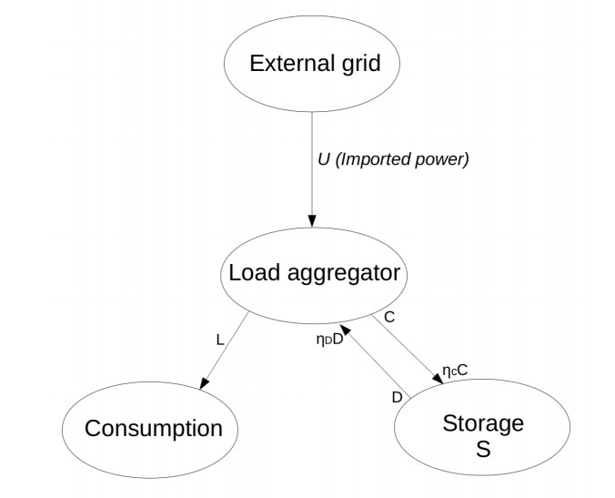
This work is devoted to study optimization problems arising in energy distribution systems with storage. We consider a simplified network topology organized around four nodes: the load aggregator, the external grid, the consumption and the storage. The imported power from the external grid should balance the consumption and the storage variation. The merit function to minimize is the total price the load aggregator has to pay in a given time interval to enforce this balance.
Two optimization problems are considered. The first one is linear and standard. It can be solved through classical optimization methods. The second problem is obtained from the previous one by taking into account a power subscription, which makes it piecewise linear. We establish mathematical properties on both these models.
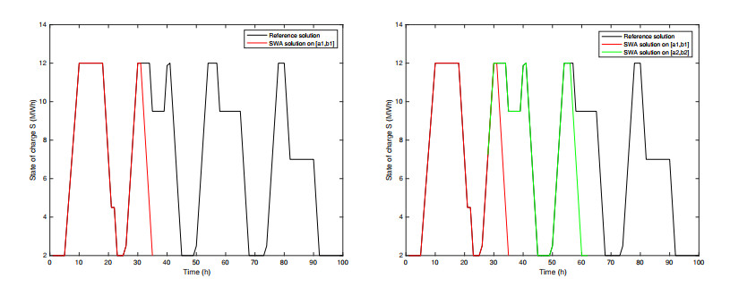
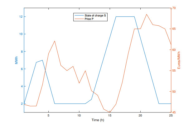
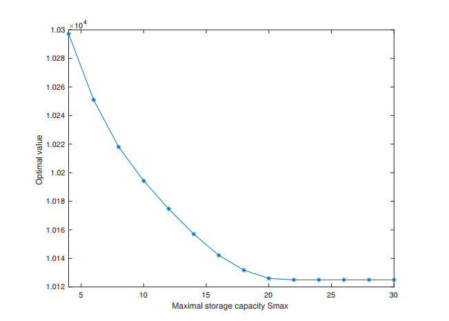
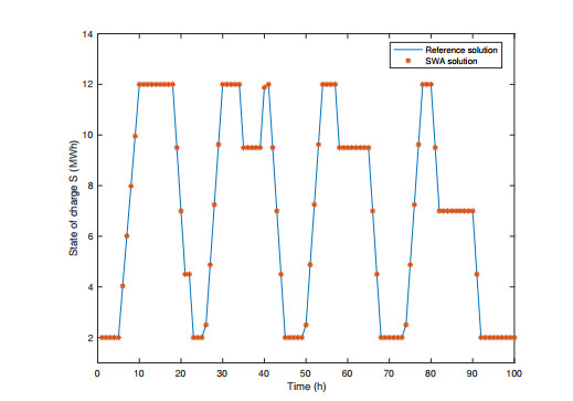
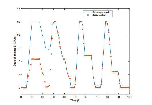
Finally, a new method based on a sliding window algorithm is derived. It allows to reduce drastically the computational time and makes feasible real time simulations. Numerical results are performed on real data to highlight both models and to illustrate the performance of the sliding window algorithm.
Citation: Jean-Paul Chehab, Vivien Desveaux, Marouan Handa. A sliding window algorithm for energy distribution system with storage[J]. AIMS Mathematics, 2021, 6(11): 11815-11836. doi: 10.3934/math.2021686
This work is devoted to study optimization problems arising in energy distribution systems with storage. We consider a simplified network topology organized around four nodes: the load aggregator, the external grid, the consumption and the storage. The imported power from the external grid should balance the consumption and the storage variation. The merit function to minimize is the total price the load aggregator has to pay in a given time interval to enforce this balance.
Two optimization problems are considered. The first one is linear and standard. It can be solved through classical optimization methods. The second problem is obtained from the previous one by taking into account a power subscription, which makes it piecewise linear. We establish mathematical properties on both these models.
Finally, a new method based on a sliding window algorithm is derived. It allows to reduce drastically the computational time and makes feasible real time simulations. Numerical results are performed on real data to highlight both models and to illustrate the performance of the sliding window algorithm.

| [1] | J. F. Bonnans, J. C. Gilbert, C. Lemaréchal, C. A. Sagastizábal, Numerical optimization: Theoretical and practical aspects, Springer Science & Business Media, 2006. |
| [2] | S. Boyd, S. P. Boyd, L. Vandenberghe, Convex optimization, Cambridge university press, 2004. |
| [3] |
T. Chen, Y. Jin, H. Lv, A. Yang, M. Liu, B. Chen, et al. Applications of lithium-ion batteries in grid-scale energy storage systems, Trans. Tianjin Univ., 26 (2020), 208–217. doi: 10.1007/s12209-020-00236-w

|
| [4] | U. D. E. A. Committee, Bottling electricity: Storage as a strategic tool for managing variability and capacity concerns in the modern grid, tech. rep., 2008. |
| [5] | M. Drouin, H. Abou-Kandil, M. Mariton, Basic concepts of discrete-time optimal control theory, In: Control of Complex Systems, Springer, 1991, 11–38. |
| [6] | J. Eyer, G. Corey, Energy storage for the electricity grid: Benefits and market potential assessment guide, Sandia Nat. Laboratories, 20 (2010), 5. |
| [7] |
I. Keppo, M. Strubegger, Short term decisions for long term problems–the effect of foresight on model based energy systems analysis, Energy, 35 (2010), 2033–2042. doi: 10.1016/j.energy.2010.01.019
|
| [8] | B. Kouvaritakis, M. Cannon, Model predictive control, Switzerland: Springer International Publishing, (2016), 38. |
| [9] |
Y. Lee, K. Tay, Y. Choy, Forecasting electricity consumption using time series model, Int. J. Eng. Technol., 7 (2018), 218–223. doi: 10.14419/ijet.v7i4.30.22363
|
| [10] |
J. F. Marquant, R. Evins, J. Carmeliet, Reducing computation time with a rolling horizon approach applied to a milp formulation of multiple urban energy hub system, Procedia Comput. Sci., 51 (2015), 2137–2146. doi: 10.1016/j.procs.2015.05.486
|
| [11] | F. J. Nogales, J. Contreras, A. J. Conejo, R. Espínola, Forecasting next-day electricity prices by time series models, IEEE Trans. Power Syst., 17 (2002), 342–348. |
| [12] | A. Peshkov, O. Alsova, Short-term forecasting of the time series of electricity prices with ensemble algorithms, In: Journal of Physics: Conference Series, vol. 1661, IOP Publishing, 2020, p. 012070. |
| [13] | K. Poncelet, E. Delarue, D. Six, W. D'haeseleer, Myopic optimization models for simulation of investment decisions in the electric power sector, In: 2016 13th International Conference on the European Energy Market (EEM), IEEE, 2016, 1–9. |
| [14] |
M. Rawa, A. Abusorrah, Y. Al-Turki, S. Mekhilef, M. H. Mostafa, Z. M. Ali, et al. Optimal allocation and economic analysis of battery energy storage systems: Self-consumption rate and hosting capacity enhancement for microgrids with high renewable penetration, Sustainability, 12 (2020), 10144. doi: 10.3390/su122310144
|
| [15] |
J. Su, T. Lie, R. Zamora, A rolling horizon scheduling of aggregated electric vehicles charging under the electricity exchange market, Appl. Energy, 275 (2020), 115406. doi: 10.1016/j.apenergy.2020.115406
|
| [16] |
Y. Xu, C. Singh, Adequacy and economy analysis of distribution systems integrated with electric energy storage and renewable energy resources, IEEE Trans. Power Syst., 27 (2012), 2332–2341. doi: 10.1109/TPWRS.2012.2186830
|
| [17] | Y. Xu, C. Singh, Power system reliability impact of energy storage integration with intelligent operation strategy, IEEE Trans. Smart Grid, 5 (2013), 1129–1137. |
| [18] | Y. Xu, L. Xie, C. Singh, Optimal scheduling and operation of load aggregators with electric energy storage facing price and demand uncertainties, In: 2011 North American Power Symposium, IEEE, 2011, 1–7. |
Figures(10) / Tables(5)

Jean-Paul Chehab, Vivien Desveaux, Marouan Handa. A sliding window algorithm for energy distribution system with storage[J]. AIMS Mathematics, 2021, 6(11): 11815-11836. doi: 10.3934/math.2021686


 DownLoad: