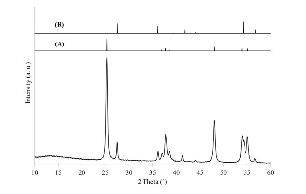
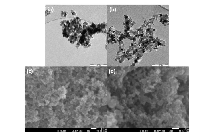
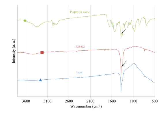
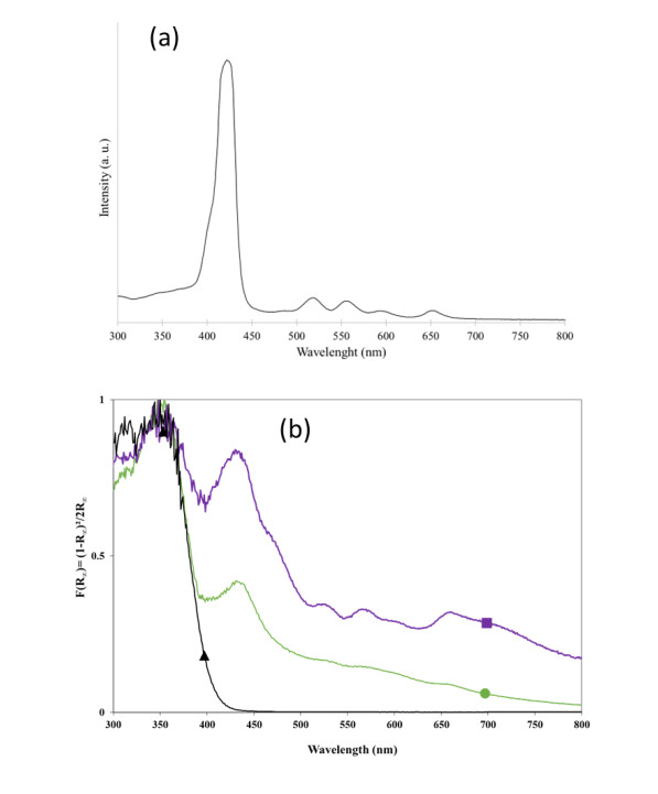
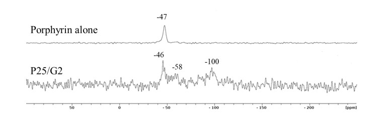
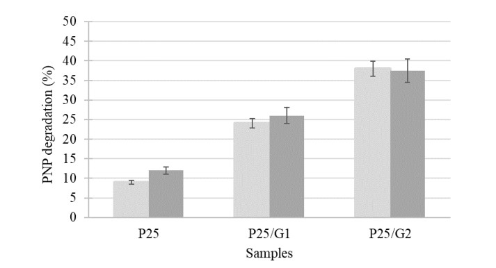
An Evonik P25 TiO2 material is modified using a porphyrin containing Si-(OR)3 extremities to extend its absorption spectrum in the visible range. Two different loadings of porphyrin are grafted at the surface of P25. The results show that the crystallinity and the texture of the P25 are not modified with the porphyrin grafting and the presence of the latter is confirmed by Fourier-transform infrared spectroscopy (FTIR) measurements. All three samples are composed of anatase/rutile titania nanoparticles around 20 nm in size with a spherical shape. The absorption spectra of the porphyrin modified samples show visible absorption alongside the characteristic Soret and Q bands of porphyrin, despite slightly shifted peak values. The 29Si solid state nuclear magnetic resonance (NMR) spectra show that the porphyrin is linked with Ti–O–C and Ti–O–Si bonds with the Evonik P25, allowing for a direct electron transfer between the two materials. Finally, the photoactivity of the materials is assessed on the degradation of a model pollutant—p-nitrophenol (PNP)—in water. The degradation is substantially enhanced when the porphyrin is grafted at its surface, whereas a very low activity is evidenced for P25. Indeed, with the best sample, the activity increases from 9% to 38% under visible light illumination. This improvement is due to the activation of the porphyrin under visible light that produces electrons, which are then transferred to the TiO2 to generate radicals able to degrade organic pollutants. The observed degradation is confirmed to be a mineralization of the PNP. Recycling experiments show a constant PNP degradation after 5 cycles of photocatalysis of 24 h each.
Citation: Julien G. Mahy, Carole Carcel, Michel Wong Chi Man. Evonik P25 photoactivation in the visible range by surface grafting of modified porphyrins for p-nitrophenol elimination in water[J]. AIMS Materials Science, 2023, 10(3): 437-452. doi: 10.3934/matersci.2023024
An Evonik P25 TiO2 material is modified using a porphyrin containing Si-(OR)3 extremities to extend its absorption spectrum in the visible range. Two different loadings of porphyrin are grafted at the surface of P25. The results show that the crystallinity and the texture of the P25 are not modified with the porphyrin grafting and the presence of the latter is confirmed by Fourier-transform infrared spectroscopy (FTIR) measurements. All three samples are composed of anatase/rutile titania nanoparticles around 20 nm in size with a spherical shape. The absorption spectra of the porphyrin modified samples show visible absorption alongside the characteristic Soret and Q bands of porphyrin, despite slightly shifted peak values. The 29Si solid state nuclear magnetic resonance (NMR) spectra show that the porphyrin is linked with Ti–O–C and Ti–O–Si bonds with the Evonik P25, allowing for a direct electron transfer between the two materials. Finally, the photoactivity of the materials is assessed on the degradation of a model pollutant—p-nitrophenol (PNP)—in water. The degradation is substantially enhanced when the porphyrin is grafted at its surface, whereas a very low activity is evidenced for P25. Indeed, with the best sample, the activity increases from 9% to 38% under visible light illumination. This improvement is due to the activation of the porphyrin under visible light that produces electrons, which are then transferred to the TiO2 to generate radicals able to degrade organic pollutants. The observed degradation is confirmed to be a mineralization of the PNP. Recycling experiments show a constant PNP degradation after 5 cycles of photocatalysis of 24 h each.

| [1] |
Turolla A, Fumagalli M, Bestetti M, et al. (2012) Electrophotocatalytic decolorization of an azo dye on TiO2 self-organized nanotubes in a laboratory scale reactor. Desalination 285:377–382. https://doi.org/10.1016/j.desal.2011.10.029 doi: 10.1016/j.desal.2011.10.029

|
| [2] |
Oturan MA, Aaron JJ (2014) Advanced oxidation processes in water/wastewater treatment: Principles and applications. A review. Crit Rev Environ Sci Technol 44: 2577–2641. https://doi.org/10.1080/10643389.2013.829765 doi: 10.1080/10643389.2013.829765
|
| [3] |
Mahy JG, Wolfs C, Mertes A, et al. (2019) Advanced photocatalytic oxidation processes for micropollutant elimination from municipal and industrial water. J Environ Manage 250: 109561. https://doi.org/10.1016/j.jenvman.2019.109561 doi: 10.1016/j.jenvman.2019.109561
|
| [4] |
Mahy JG, Wolfs C, Vreuls C, et al. (2021) Advanced oxidation processes for wastewater treatment: From lab-scale model water to on-site real waste water. Environ Technol 42: 3974–3986. https://doi.org/10.1080/09593330.2020.1797894 doi: 10.1080/09593330.2020.1797894
|
| [5] |
Baaloudj O, Nasrallah N, Kebir M, et al. (2021) A comparative study of ceramic nanoparticles synthesized for antibiotic removal: catalysis characterization and photocatalytic performance modeling. Environ Sci Pollut R 28: 13900–13912. https://doi.org/10.1007/s11356-020-11616-z/Published doi: 10.1007/s11356-020-11616-z/Published
|
| [6] |
Baaloudj O, Nasrallah N, Bouallouche R, et al. (2022) High efficient Cefixime removal from water by the sillenite Bi12TiO20: Photocatalytic mechanism and degradation pathway. J Clean Prod 330: 12994. https://doi.org/10.1016/j.jclepro.2021.129934 doi: 10.1016/j.jclepro.2021.129934
|
| [7] | Fujishima A, Hashimoto K, Watanabe T (1999) TiO2 Photocatalysis: Fundamentals and Applications, BKC. |
| [8] |
Rauf MA, Ashraf SS (2009) Fundamental principles and application of heterogeneous photocatalytic degradation of dyes in solution. Chem Eng J 151: 10–18. https://doi.org/10.1016/j.cej.2009.02.026 doi: 10.1016/j.cej.2009.02.026
|
| [9] |
Mahy JG, Léonard GL-M, Pirard S, et al. (2017) Aqueous sol-gel synthesis and film deposition methods for the large-scale manufacture of coated steel with self-cleaning properties. J Sol-gel Sci Technol 81: 27–35. https://doi.org/10.1007/s10971-016-4020-5 doi: 10.1007/s10971-016-4020-5
|
| [10] |
Malengreaux CM, Douven S, Poelman D, et al. (2014) An ambient temperature aqueous sol-gel processing of efficient nanocrystalline doped TiO2-based photocatalysts for the degradation of organic pollutants. J Sol-gel Sci Technol 71: 557–570. https://doi.org/10.1007/s10971-014-3405-6 doi: 10.1007/s10971-014-3405-6
|
| [11] |
Todorova N, Giannakopoulou T, Karapati S, et al. (2014) Composite TiO2/clays materials for photocatalytic NOx oxidation. Appl Surf Sci 319: 113–120. https://doi.org/10.1016/j.apsusc.2014.07.020 doi: 10.1016/j.apsusc.2014.07.020
|
| [12] |
Romeiro A, Azenha ME, Canle M, et al. (2018) Titanium dioxide nanoparticle photocatalysed degradation of ibuprofen and naproxen in water: Competing hydroxyl radical attack and oxidative decarboxylation by semiconductor holes. ChemistrySelect 3: 10915–10924. https://doi.org/10.1002/slct.201801953 doi: 10.1002/slct.201801953
|
| [13] |
Mbouopda AP, Acayanka E, Nzali S, et al. (2018) Comparative study of plasma-synthesized and commercial-P25 TiO2 for photocatalytic discoloration of reactive Red 120 dye in aqueous solution. Desalination Water Treat 136: 413–421. https://doi.org/10.5004/dwt.2018.23118 doi: 10.5004/dwt.2018.23118
|
| [14] |
Mahy JG, Tilkin RG, Douven S, et al. (2019) TiO2 nanocrystallites photocatalysts modified with metallic species: Comparison between Cu and Pt doping. Surf Interface 17: 100366. https://doi.org/10.1016/j.surfin.2019.100366 doi: 10.1016/j.surfin.2019.100366
|
| [15] |
Mahy JG, Lambert SD, Tilkin RG, et al. (2019) Ambient temperature ZrO2-doped TiO2 crystalline photocatalysts: Highly efficient powders and films for water depollution. Mater Today Energy 13: 312–322. https://doi.org/10.1016/j.mtener.2019.06.010 doi: 10.1016/j.mtener.2019.06.010
|
| [16] |
Douven S, Mahy JG, Wolfs C, et al. (2020) Efficient N, Fe Co-doped TiO2 active under cost-effective visible LED light: From powders to films. Catalysts 10: 547. https://doi.org/10.3390/catal10050547 doi: 10.3390/catal10050547
|
| [17] |
Impellizzeri G, Scuderi V, Romano L, et al. (2016) Fe ion-implanted TiO2 thin film for efficient visible-light photocatalysis Fe ion-implanted TiO2 thin film for efficient visible-light photocatalysis. J Appl Phys 116: 173507. https://doi.org/10.1063/1.4901208 doi: 10.1063/1.4901208
|
| [18] |
Espino-estévez MR, Fernández-rodríguez C, González-díaz OM (2016) Effect of TiO2-Pd and TiO2-Ag on the photocatalytic oxidation of diclofenac, isoproturon and phenol. Chem Eng J 298: 82–95. https://doi.org/10.1016/j.cej.2016.04.016 doi: 10.1016/j.cej.2016.04.016
|
| [19] |
Mahy JG, Cerfontaine V, Poelman D, et al. (2018) Highly efficient low-temperature N-doped TiO2 catalysts for visible light photocatalytic applications. Materials 11: 584. https://doi.org/10.3390/ma11040584 doi: 10.3390/ma11040584
|
| [20] |
Pelaez M, Nolan NT, Pillai SC, et al. (2012) A review on the visible light active titanium dioxide photocatalysts for environmental applications. Appl Catal B 125: 331–349. https://doi.org/10.1016/j.apcatb.2012.05.036 doi: 10.1016/j.apcatb.2012.05.036
|
| [21] |
Bodson CJ, Heinrichs B, Tasseroul L, et al. (2016) Efficient P- and Ag-doped titania for the photocatalytic degradation of wastewater organic pollutants. J Alloys Compd 682: 144–153. https://doi.org/10.1016/j.jallcom.2016.04.295 doi: 10.1016/j.jallcom.2016.04.295
|
| [22] |
Léonard GLM, Remy S, Heinrichs B (2016) Doping TiO2 films with carbon nanotubes to simultaneously optimise antistatic, photocatalytic and superhydrophilic properties. J Sol-gel Sci Technol 79: 413–425. https://doi.org/10.1007/s10971-016-3975-6 doi: 10.1007/s10971-016-3975-6
|
| [23] |
Léonard GL-M, Pàez CA, Ramírez AE, et al. (2018) Interactions between Zn2+ or ZnO with TiO2 to produce an efficient photocatalytic, superhydrophilic and aesthetic glass. J Photochem Photobiol A Chem 350. https://doi.org/10.1016/j.jphotochem.2017.09.036 doi: 10.1016/j.jphotochem.2017.09.036
|
| [24] |
Reinosa JJ, María C, Docio Á, et al. (2018) Hierarchical nano ZnO-micro TiO2 composites: High UV protection yield lowering photodegradation in sunscreens. Ceram Int 44: 2827–2834. https://doi.org/10.1016/j.ceramint.2017.11.028 doi: 10.1016/j.ceramint.2017.11.028
|
| [25] |
Wu M, Leung DYC, Zhang Y, et al. (2019) Toluene degradation over Mn-TiO2/CeO2 composite catalyst under vacuum ultraviolet (VUV) irradiation. Chem Eng Sci 195: 985–994. https://doi.org/10.1016/j.ces.2018.10.044 doi: 10.1016/j.ces.2018.10.044
|
| [26] |
Min KS, Kumar RS, Lee JH, et al. (2019) Synthesis of new TiO2/porphyrin-based composites and photocatalytic studies on methylene blue degradation. Dyes and Pigments 160: 37–47. https://doi.org/10.1016/j.dyepig.2018.07.045 doi: 10.1016/j.dyepig.2018.07.045
|
| [27] |
Wu T, Lin T, Serpone N (1999) TiO2-assisted photodegradation of dyes. 9. photooxidation of a squarylium cyanine dye in aqueous dispersions under visible light irradiation. Environ Sci Technol 33:1379–1387. https://doi.org/10.1021/es980923i doi: 10.1021/es980923i
|
| [28] |
Mahy JG, Paez CA, Carcel C, et al. (2019) Porphyrin-based hybrid silica-titania as a visible-light photocatalyst. J Photochem Photobiol A Chem 373: 66–76. https://doi.org/10.1016/j.jphotochem.2019.01.001 doi: 10.1016/j.jphotochem.2019.01.001
|
| [29] |
Musial J, Belet A, Mlynarczyk DT, et al. (2022) Nanocomposites of titanium dioxide and peripherally substituted phthalocyanines for the photocatalytic degradation of sulfamethoxazole. Nanomaterials 12: 3279. https://doi.org/10.3390/nano12193279 doi: 10.3390/nano12193279
|
| [30] |
Ramasubbu V, Ram Kumar P, Chellapandi T, et al. (2022) Zn(Ⅱ) porphyrin sensitized (TiO2@Cd-MOF) nanocomposite aerogel as novel photocatalyst for the effective degradation of methyl orange (MO) dye. Opt Mater132: 112558. https://doi.org/10.1016/j.optmat.2022.112558 doi: 10.1016/j.optmat.2022.112558
|
| [31] |
Yadav V, Verma P, Negi H, et al. (2023) Efficient degradation of 4-nitrophenol using VO(TPP) impregnated TiO2 photocatalyst: Insight into kinetics and mechanism. J Mater Res 38: 237–247. https://doi.org/10.1557/s43578-022-00856-z doi: 10.1557/s43578-022-00856-z
|
| [32] |
Rengifo-Herrera JA, Blanco MN, Fidalgo De Cortalezzi MM, et al. (2016) Visible-light-absorbing Evonik P-25 nanoparticles modified with tungstophosphoric acid and their photocatalytic activity on different wavelengths. Mater Res Bull 83: 360–368. https://doi.org/10.1016/j.materresbull.2016.06.026 doi: 10.1016/j.materresbull.2016.06.026
|
| [33] |
Wang L, Duan S, Jin P, et al. (2018) Anchored Cu(Ⅱ) tetra(4-carboxylphenyl)porphyrin to P25 (TiO2) for efficient photocatalytic ability in CO2 reduction. Appl Catal B 239: 599–608. https://doi.org/10.1016/j.apcatb.2018.08.007 doi: 10.1016/j.apcatb.2018.08.007
|
| [34] |
Tio N, Cherian S, Wamser CC (2000) Adsorption and photoactivity of tetra (4-carboxyphenyl) porphyrin (TCPP) on nanoparticulate TiO2. J Phys Chem B 104: 3624–3629. https://doi.org/10.1021/jp994459v doi: 10.1021/jp994459v
|
| [35] |
Kubelka P (1948) New contributions to the optics of intensely light-scattering materials. J Opt Soc Am 38:448–457. https://doi.org/10.1364/JOSA.44.000330 doi: 10.1364/JOSA.44.000330
|
| [36] |
Mahy JG, Lambert SD, Léonard GLM, et al. (2016) Towards a large scale aqueous sol-gel synthesis of doped TiO2: Study of various metallic dopings for the photocatalytic degradation of p-nitrophenol. J Photochem Photobiol A Chem 329: 189–202. https://doi.org/10.1016/j.jphotochem.2016.06.029 doi: 10.1016/j.jphotochem.2016.06.029
|
| [37] |
Thommes M, Kaneko K, Neimark A, et al. (2015) Physisorption of gases, with special reference to the evaluation of surface area and pore size distribution (IUPAC Technical Report). Pure Appl Chem 87: 1051–1069. https://doi.org/10.1515/pac-2014-1117 doi: 10.1515/pac-2014-1117
|
| [38] |
Tasseroul L, Páez CA, Lambert SD, et al. (2016) Photocatalytic decomposition of hydrogen peroxide over nanoparticles of TiO2 and Ni(Ⅱ)porphyrin-doped TiO2: A relationship between activity and porphyrin anchoring mode. Appl Catal B 182: 405–413. https://doi.org/10.1016/j.apcatb.2015.09.042 doi: 10.1016/j.apcatb.2015.09.042
|
| [39] |
Mahy JG, Douven S, Hollevoet J, et al. (2021) Easy stabilization of Evonik Aeroxide P25 colloidal suspension by 4-hydroxybenzoic acid functionalization. Surf Interface 27: 101501. https://doi.org/10.1016/j.surfin.2021.101501 doi: 10.1016/j.surfin.2021.101501
|
| [40] |
Tasseroul L, Lambert SD, Eskenazi D, et al. (2013) Degradation of p-nitrophenol and bacteria with TiO2 xerogels sensitized in situ with tetra(4-carboxyphenyl) porphyrins. J Photochem Photobiol A Chem 272: 90–99. https://doi.org/10.1016/j.jphotochem.2013.08.023 doi: 10.1016/j.jphotochem.2013.08.023
|
| [41] |
Tasseroul L, Pirard SL, Lambert SD, et al. (2012) Kinetic study of p-nitrophenol photodegradation with modified TiO2 xerogels. Chem Eng J 191: 441–450. https://doi.org/10.1016/j.cej.2012.02.050 doi: 10.1016/j.cej.2012.02.050
|
| [42] |
Cerneaux S, Zakeeruddin SM, Pringle JM, et al. (2007) Novel nano-structured silica-based electrolytes containing quaternary ammonium iodide moieties. Adv Funct Mater 17: 3200–3206. https://doi.org/10.1002/adfm.200700391 doi: 10.1002/adfm.200700391
|
| [43] |
Corriu RJP, Moreau JJE, Thepot P, et al. (1992) New mixed organic-inorganic polymers: Hydrolysis and polycondensation of bis(trimethoxysilyl) organometallic precursors. Chem Mater 4: 1217–1224. https://doi.org/10.1021/cm00024a020 doi: 10.1021/cm00024a020
|
| [44] |
Chan Y-J, Kum B-G, Park Y-C, et al. (2014) Surface modification of TiO2 nanoparticles with phenyltrimethoxysilane in dye-sensitized solar cells. Bull Korean Chem Soc 35: 415–418. https://doi.org/10.5012/bkcs.2014.35.2.415 doi: 10.5012/bkcs.2014.35.2.415
|
| [45] |
Kathiravan A, Renganathan R, Anandan S (2010) Electron transfer dynamics from the singlet and triplet excited states of meso-tetrakis (p-carboxyphenyl) porphyrin into colloidal. J Colloid Interface Sci 348: 642–648. https://doi.org/10.1016/j.jcis.2010.05.002 doi: 10.1016/j.jcis.2010.05.002
|
| [46] |
Baaloudj O, Assadi AA, Azizi M, et al. (2021) Synthesis and characterization of ZnBi2O4 nanoparticles: Photocatalytic performance for antibiotic removal under different light sources. Appl Sci-Basel 11: 3975. https://doi.org/10.3390/app11093975 doi: 10.3390/app11093975
|
| [47] |
Paola A Di, Augugliaro V, Palmisano L, et al. (2003) Heterogeneous photocatalytic degradation of nitrophenols. J Photochem Photobiol A Chem 155: 207–214. https://doi.org/10.1016/S1010-6030(02)00390-8 doi: 10.1016/S1010-6030(02)00390-8
|
| [48] |
Augugliaro V, Palmisano L, Schiavello M, et al. (1991) Photocatalytic degradation of nitrophenols in aqueous titanium dioxide dispersion. Appl Catal 69: 323–340. https://doi.org/http://dx.doi.org/10.1016/S0166-9834(00)83310-2 doi: 10.1016/S0166-9834(00)83310-2
|
 matersci-10-03-024-s001.pdf matersci-10-03-024-s001.pdf |
 |
Figures(6) / Tables(3)

Julien G. Mahy, Carole Carcel, Michel Wong Chi Man. Evonik P25 photoactivation in the visible range by surface grafting of modified porphyrins for p-nitrophenol elimination in water[J]. AIMS Materials Science, 2023, 10(3): 437-452. doi: 10.3934/matersci.2023024


 DownLoad: