Biochar in cementitious material—A review on physical, chemical, mechanical, and durability properties

Pravina Kamini G.; Kong Fah Tee; Jolius Gimbun; Siew Choo Chin; Pravina Kamini G.; Kong Fah Tee; Jolius Gimbun; Siew Choo Chin

doi:10.3934/matersci.2023022

AIMS Materials Science

2023, Volume 10, Issue 3: 405-425. doi: 10.3934/matersci.2023022

Previous Article Next Article

Review

Biochar in cementitious material—A review on physical, chemical, mechanical, and durability properties

1.
Faculty of Civil Engineering Technology, Universiti Malaysia Pahang, 26300 Gambang, Malaysia
2.
Department of Civil and Environmental Engineering, King Fahd University of Petroleum and Minerals, Dhahran 31261, Saudi Arabia
3.
Interdisciplinary Research Center for Construction and Building Materials, KFUPM, Dhahran 31261, Saudi Arabia
4.
Center of Research in Advance Fluid and Process (Fluid Center), Universiti Malaysia Pahang, 26300 Gambang, Malaysia
5.
Faculty of Chemical and Process Engineering Technology, Universiti Malaysia Pahang, 26300 Gambang, Malaysia

Received: 15 December 2022 Revised: 21 March 2023 Accepted: 09 April 2023 Published: 06 May 2023

Ordinary Portland Cement (OPC) is a crucial building component and a valuable strategic resource. The production of cement accounts for 5% to 10% of global carbon dioxide (CO₂) emissions. Over the years, many researchers have been studying ways to reduce the amount of CO₂ in the atmosphere caused by cement production. Due to its properties, biochar is found to be an interesting material to be utilised in the construction industry due to its effectiveness in CO₂ sequestration. Biochar is a solid residue created by the thermal breakdown of biomass at moderate temperatures (350–700 ℃) without oxygen or with a small amount of oxygen, sometimes known as bio-carbon. Biochar has a wide range of uses, including those for heating and electricity generation, cleaning flue gases, metallurgy, animal husbandry, agriculture, construction materials, and even medicine. The objective of this paper is to review the potential of biochar as a cementitious material by evaluating its physical, chemical, mechanical, and durability properties. Using biochar as a cementitious material makes it possible to conclude that cement production will be reduced over time by partial replacement, which will also promote and encourage sustainable development in the future.

Keywords:

Citation: Pravina Kamini G., Kong Fah Tee, Jolius Gimbun, Siew Choo Chin. Biochar in cementitious material—A review on physical, chemical, mechanical, and durability properties[J]. AIMS Materials Science, 2023, 10(3): 405-425. doi: 10.3934/matersci.2023022

Related Papers:

[1]	Jawad Saleemi . COVID-19 and liquidity risk, exploring the relationship dynamics between liquidity cost and stock market returns. National Accounting Review, 2021, 3(2): 218-236. doi: 10.3934/NAR.2021011
[2]	Yanting Xu, Tinghui Li . Measuring digital economy in China. National Accounting Review, 2022, 4(3): 251-272. doi: 10.3934/NAR.2022015
[3]	Jiehua Ma, Zhenghui Li . Measuring China's urban digital economy. National Accounting Review, 2022, 4(4): 329-361. doi: 10.3934/NAR.2022019
[4]	Rashesh Vaidya . NEPSE in Bollinger Bands. National Accounting Review, 2021, 3(4): 439-451. doi: 10.3934/NAR.2021023
[5]	Mustafa Tevfik Kartal . Do activities of foreign investors affect main stock exchange indices? Evidence from Turkey before and in time of Covid-19 pandemic. National Accounting Review, 2020, 2(4): 384-401. doi: 10.3934/NAR.2020023
[6]	Lanli Hu, Yaqi Gong, Lu Zhu . The impact of new digital infrastructure on total factor productivity in the education service industry: evidence from China. National Accounting Review, 2025, 7(3): 309-339. doi: 10.3934/NAR.2025014
[7]	Cheng Li . Unequal wealth of nations: Evidence from the World Bank wealth accounts. National Accounting Review, 2024, 6(3): 384-406. doi: 10.3934/NAR.2024018
[8]	Jinhui Zhu, Mengxin Wang, Changhong Zhang . Impact of high-standard basic farmland construction policies on agricultural eco-efficiency: Case of China. National Accounting Review, 2022, 4(2): 147-166. doi: 10.3934/NAR.2022009
[9]	Tinghui Li, Zimei Huang, Benjamin M Drakeford . Statistical measurement of total factor productivity under resource and environmental constraints. National Accounting Review, 2019, 1(1): 16-27. doi: 10.3934/NAR.2019.1.16
[10]	María-José Murgui-García, Jose-Ramon Ruiz-Tamarit . Economic resilience in the short-run: A dynamic macroeconomic approach. National Accounting Review, 2025, 7(3): 290-308. doi: 10.3934/NAR.2025013

Abstract

1. Introduction

In most problems solved in the field of measuring technology, radar, astronomy, optical communication, positioning, navigation, television automation and many other broad areas of science and technology, one of the fundamental problems is finding the best way to recognize a signal in the presence of interference. The ideal reception of signals under the influence of noise and interference is based on simple yet deep ideas, set out in the most consistent and understandable form by Woodward (Woodward, 1955). Following this idea, the task of an ideal device, whose input receives a mixture of signal with noise, is the complete removal of unnecessary information contained in this mixture, and the preservation of useful information about those signal parameters that are of interest to the system user.

The task of calculating composite indicators characterizing the quality of a system can also be attributed to the problems of signal isolation against a background of interference. Comparison of the considered objects' integral indicators and ratings generated by their composite indices, makes it possible to judge the degree of achievement of the management objective. Although the scientific community has not come to a common opinion, if it is possible in principle to characterize a multifaceted phenomenon as a single scalar. International organizations, think tanks and social sciences at the turn of the millennium significantly increased the number of integrated indicators used to measure various latent characteristics of social and economic systems: social capital, human development, quality of life, quality of management, etc.

According to the UN, by 2011 there were 290 indices developed for the ranking or integrated assessment of countries. A review of the phenomenal growth in the number of complex indexes used by countries for integrated assessment performed by Bandura (Bandura, 2006, 2008, 2011) showed that only 26 of them (9%) were formed before 1991,132 (46%) from 1991 to 2006, and 130 consolidated indices were formed in the period 2007–2011. A huge number of methods used to assess the latent characteristics of social systems highlight the dissatisfaction with the results and the need for further research in this area.

The rapid increase in the number of complex indexes is a clear sign of their importance in politics and the economy. All major international organizations, such as the Organization for Economic Cooperation and Development (OECD), the European Union, the World Economic Forum or the International Monetary Fund, are constructing composite indicators in various fields (Bandura, 2011; Nardo et al., 2005). The overall goal of most of these indicators is the ranking of objects (countries) and their comparative analysis for some agammaegate measure (Bandura, 2011; Foa and Tanner, 2012; Saltelli et al., 2006; Sharpe, 2004). The use of a single indicator characterizing poorly formalized processes of social systems (quality of life, demographic situation, etc.) is the only possible solution to this problem. Therefore, improving the quality of composite indicators is relevant both from a theoretical and from a practical point of view. A discussion of the pros and cons of composite indicators is given in (Nardo et al., 2005; Foa and Tanner, 2012).

Despite the huge number of used composite indicators, unresolved methodological problems in their design lead to the fact that very often they raise more questions than they give answers. The huge number of applied methods for assessing the latent characteristics of social systems indicates the dissatisfaction of researchers with the results and the need for further research in this area.

The Organization for Economic Cooperation and Development (OECD) is constantly working to improve the methods for constructing complex indexes (Nardo et al., 2005; Saltelli et al., 2006; Nicoletti et al., 2000; Saltelli, 2007). In 2008, the OECD, together with the Joint Research Center of the European Commission, prepared a (Handbook, 2008), which was the result of years of research in this field (Nardo et al., 2005; Saltelli et al., 2006; Nicoletti et al., 2000, Saltelli, 2007; Tarantola et al., 2002). The Handbook sets out a set of technical principles for the formation of composite indices. The authors choose a linear convolution of indicators for the primary method of the data's agammaegation, while the main tool for constructing composite indicators is factor analysis.

So, to build a qualitative integral indicator, it is required: first, a thorough theoretical study of the measured phenomena's theoretical aspects, since "that which is not well defined is likely to be poorly measured" (Nardo et al., 2005), secondly, the choice of data quality, because the quality of the composite indicators largely depends on the quality of the main indicators and, thirdly, an adequate tool for working with multidimensional data.

Such a tool for working with multidimensional data is multidimensional statistical data analysis, namely, factor analysis and principal component analysis (PCA). Factor analysis was first used to combine a multitude of indicators into a single index in the development of the Health Index by (Hightower, 1978).

When calculating Socio-Economic Status Indices (SES), the principal component analysis was adopted as a standard for the construction method, and the calculated index was determined with a projection onto the first principal component (McKenzie, 2005; Vyas S and Kumaranayake, 2006). The same methodology was used by Lindman and Selin in creating the Environmental Sustainability Index (Lindman and Selin, 2011). Somarriba and Penna used PCA in measuring the quality of life in Europe (Somarriba and Pena, 2009). Mention should also be made of (Ajvazjan, 2003) on the definition of a population's quality of life index using the first principal component.

However, the first principal component approximates the simulated situation well if the maximum eigenvalue of the covariance matrix contributes at least 70% to the sum of all eigenvalues. This relationship is satisfied if a small number of features are considered (no more than five), and one of the properties of the system clearly dominates over the others. When describing socio-economic systems, the number of variables significantly exceeds five, and the structure of the system does not allow simple approximation. As a way out of this situation, according to (Ajvazjan, 2003), the information threshold is reduced to 55%, and the system is divided into subsystems described with a smaller number of variables. In the studies discussed above (Hightower, 1978; McKenzie, 2005; Vyas and Kumaranayake, 2006; Somarriba and Pena, 2009), the contribution of the largest eigenvalue ranged from 13% to 38%, with the exception of (Somarriba and Pena, 2009), in which an example of a model was considered, where this figure was 56%.

The authors followed the recommendations (Somarriba and Pena, 2009), which stated that the first principal component gives satisfactory weight coefficients when calculating the integral index even in cases where the largest eigenvalue makes a small contribution to the sum of all eigenvalues. However, such a statement cannot be called indisputable. In the study (Mazziotta and Pareto, 2016) the contribution of the largest eigenvalue of 74% the authors consider insufficient.

For a fixed t an integrated assessment is often recorded for each of the object numbered i in the form of additive data convolution with some weights. Researchers at the Organization for Economic Cooperation and Development hold a different point of view. For the formation of a composite index, factor analysis is used, where the analysis of the first principal components is used exclusively for extracting factors, so that the number of factors extracted explains more than 50% of the total variance. The value of the composite index in this case is determined only with significant loads of the selected main factors after rotation. De facto, this method becomes the standard for calculating complex indexes (Nardo et al., 2005; Nicoletti et al., 2000; Tarantola et al., 2002). Although the authors of (Nardo et al., 2005) pay attention to the fact that different methods of extracting the principle components and different methods of rotation imply different significant variables and, therefore, different weights of variables when calculating the composite index, hence different values of the calculated integral indicator. In addition, factor analysis assumes there is sufficient correlation between the initial variables, which to some extent contradicts the idea of a complete description of the phenomenon under study by a set of independent variables.

Another circumstance should also be noted. Methods for determining weight coefficients using factor analysis cannot be used to compare the characteristics of objects described in dynamics. For different observations, the structure of factors is different, even for fixed methods of extracting factors and the rotation process. This makes intertemporal comparison meaningless (Zhgun, 2013). The reason for the different structure of the main factors may be the insufficient quality of the data used, namely the presence of errors in the data. Nevertheless, it is the statistical data containing fatal errors that currently represent the best estimates of the available real values in social systems (Nardo et al., 2005).

It is impossible to obtain exact characteristics of an object based on a single measurement, which inevitably contains an unknown error. However, based on a series of such measurements, it is possible to calculate the unknown characteristic. In particular, astrophotometry successfully solves this problem. It determines the basic numerical parameters of astronomical objects not on a single observation (image), but on a series of noisy images. Using the basic ideas underlying astrophotometry, we consider the construction of the complex indices changes in the quality of a complex system as a solution to the problem selection of the useful signal on a series of observations containing a description of the unknown parameter (in a multidimensional dataset with noise) with a priori uncertainty of the desired signals' properties based on a specified signal-to-noise ratio.

The goal of this manuscript is to construct a composite system quality index as a solution to the problem of extracting a signal against a background of noise. For this it is suggested to take linear convolution weights as the characteristics of a system's structure. While in order to determine the structure of the system according to a series of observations a modification of the PCA for a noisy signal is proposed. Further the stability and reliability of the composite index obtained is investigated.

2. Calculation of the integrated system indicator for a series of observations

To solve the control problem, it is required to give a motivated estimate of each observed object on the entire observation interval, i.e. to calculate in dynamics the integral characteristic of system quality according to the results of available measurements. Let's consider the construction of an integral estimation of a system of m objects for which tables of n descriptions of those objects for a series of observations are known. For each moment t the vector of integral indicators is written as

$q{\, ^{t\;}}\; = \;A{\kern 1pt} {\, ^t} \cdot w{\, ^t}$

(1)

For a fixed t an integrated assessment is often recorded for each of the object numbered i in the form of additive data convolution with some weights

${q_i} = \sum\limits_{j = 1}^n {{w_j}} \cdot {a_{ij}}, \quad i = 1, 2, \quad m$

(2)

where q^t = ( q₁^t, q₂^t, …, q_m^t^,)^T —is the vector of integral indicators of the moment t, q^t—is the vector of the weights for the moment t, and A^t — is the data matrix for the time t. The numerical characteristics of the system are preliminarily subjected to unification—the reduction of the variables' values to the interval [0, 1]. If the initial indicator is related to the analyzed integral quality feature by monotone function, their putting to the interval [0, 1] will transform the variables x_ij for each time point of observation according to the rule:

${a_{i{\kern 1pt} j}}\, = \;\, {s_j}{\kern 1pt} + {\kern 1pt} {\kern 1pt} \left({ - 1} \right){{\kern 1pt} ^{{s_j}}} \cdot \frac{{{x_{ij}} - {\kern 1pt} \, {m_j}}}{{{M_j}\, - {m_j}}},$

(3)

where s_j = 0 if the optimal value of the j-th index is maximum and s_j = 1 if the optimum value of j-th index is minimal and

${M_j} = \mathop {max }\limits_{\begin{array}{*{20}{c}} {1 \le i \le n}\\ {1 \le t \le T} \end{array}} x_{ij}^t, \quad {m_j} = \mathop {min }\limits_{\begin{array}{*{20}{c}} {1 \le i \le n}\\ {1 \le t \le T} \end{array}} x_{ij}^t.$

(4)

m_j – minimum value of the j-th index for the whole sample (global minimum), M_j – maximum value of j-th index for the whole sample (global maximum). In case where there is another optimal (not minimum or maximum) index value, the following formula is used:

${a_{i{\kern 1pt} j}} = \left({1\;\; - \quad \frac{{\, \left| {{x_{ij}} - {x_j}^{opt}\, } \right|}}{{{\rm{max}}\, (({\kern 1pt} {M_j} - {x_j}^{opt}\, ), (\, {x_j}^{opt} - {m_j}\, ))}}} \right).$

(5)

To build an integral indicator of the systems' quality, it is required to find weights w_t for each time point. The method of expert assessments for determining weights is widely used due to the ease of obtaining information. However, not every complex system has a sufficient number of qualified experts. In addition, expert services are a commodity, so they are not cheap and cannot be objective. It is preferred to use formal methods that do not use human preferences (Nardo et al., 2005; Nicoletti et al., 2000; Ajvazjan, 2003). On the other hand, the extent of the importance (weights) of the variables calculated using formal methods often does not coincide with the intentions of the developers. Therefore, the weights are carefully investigated. (Becker et al., 2017a, 2017b; Paruolo et al., 2013).

The Principal Components Analysis (PCA) is perhaps the most-used method to obtain weights intrinsically. However, the application of this technique gives unexpected results. For example, in a study (Molchanova et al., 2014), the quality of life is determined by PCA (Ajvazjan, 2003). Obviously, geographically close regions should have comparable quality of life ratings. For example, Novgorod and Pskov are neighboring constitute entities and close in all parameters. However, the rating of the Novgorod province is 29, while the rating of the Pskov province is 54 (out of 83 positions). It is also obvious that the quality of life near a megapolis is higher than in Siberia and the Far East. Nevertheless, the rating of the Leningrad province is 63, lower than the ratings of Novgorod and Pskov provinces, almost as low as the rating of Sakhalin 64. Complex indices, that give such ratings, cannot be called reliable.

If technique PCA is applied to a series of observations made at different times, then, in the condition of a stable situation, the ratings have strong fluctuations (Gajdamak and Hohlov, 2009). In this case as well, the complex indices, that determine such ratings, cannot be called reliable. The numerical evaluation of such changes for (Gajdamak and Hohlov, 2009) is given further in paragraph 3.

In the paper (Mazziotta and Pareto, 2016) the authors consider that PCA is a blindly empiricist method based on the observed correlations and it ignores the polarity of the individual indicators. Therefore, if the normalized indicators are not all positively intercorrelated, the results are not correct. It should be noted that the amount of variance accounted for, and the weights computed by PCA change over time, so the results of different PCAs are not easily comparable. Consequently, they believe the use of PCA for the construction of composite indices for assessing multidimensional phenomena is at all improper. It should be noted that this conclusion was made when constructing a composite index for a single observation.

However, any measurement, including statistical, is determined by the accuracy of the measuring device, therefore the measurement result always contains an unavoidable error. The construction of system's integral characteristic can be considered as the task of isolating a useful signal against a noisy background. This problem is analogous to the problem of restoring digital images distorted by Gaussian noise. The principal component analysis makes it possible to isolate the structure in a noisy array of data and it is successfully used to reduce noise in image restoration.

The quantitative characteristics of a particular system, related to its structural features, depend on the signal-to-noise ratio. SNR—signal-to-noise ratio (SNR) is the ratio of the signal (more precisely, the sum of the signal and noise) to noise. The value is calculated either as a dimensionless ratio of the signal amplitude to the noise amplitude SNR = A_s / A_n, or, in decibels, SNR (dB) = 20 log ₁₀ (A_s / A_n).

This ratio most fully describes the quality of the signal in technical systems: television, in means of control and diagnostics, in mobile communication systems, in astrophotometry, etc. This ratio most fully describes the signal quality in technical systems: television, in control and diagnostic tools, in mobile communication systems, in astrophotometry, etc. The choice of the SNR threshold value, which makes it possible to distinguish a signal against noise is justified (Zhgun, 2014).

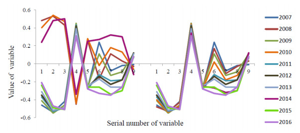
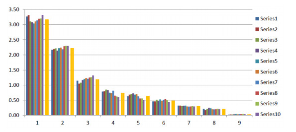
Moving to another point in time means a change in the data, which is caused by both a change in the situation and random errors. The analysis of the principal components based on different values (for consecutive moments) of eigenvectors and eigenvalues describes the invariable structure of the system. Therefore, the undistorted values of the eigenvalues and eigenvectors will be a signal that must be extracted from the noisy data. For eigenvalues, such a signal is the average. Averaging works on the assumption that the noise is absolutely random. Such averaging of the values is used in astrophotography for noise suppression. The assumption that there is a general trend in the variation of input data is illustrated in Figure 1, where the values of the covariance matrices ordered in descending eigenvalues for different observations are presented. In the mean, a tendency (signal) and a deviation from it (noise) are clearly visible.

Figure 1. The eigenvalues of the covariance matrix of the variables for different observation times. Right yellow color is the mean of the eigenvalues. The variables considered are from the first block of Table 2. Source: Rosstat // http://www.gks.ru.

DownLoad: Full-Size Img PowerPoint

The eigenvectors in the PCA are determined up to the direction, in contrast to the eigenvalues, which are uniquely determined. The mean value of variables' factor loadings depends on the chosen direction and cannot unambiguously characterize the signal.

Based on the eigenvectors calculated for various observations (ordered in decreasing order of eigenvalues), it is necessary to recognize the random and nonrandom components of these vectors.

We assume that the nonrandom (significant) contribution of a variable to the structure of the main component is not a large value of the factor load after rotation, but an invariance of the factor load with data disturbances. A sign a variable's invariance is the signal-to-noise ratio, which is calculated from the values of this variable's factor loads. The signal amplitude is the absolute value of the mean of the load factors, the noise amplitude is the standard deviation of the load factors.

If the signal-to-noise ratio is above the threshold value, then such a variable is considered nonrandom. Otherwise, the variable characterizes the noise component of the signal and does not participate in further consideration. In Figure 2 the choice of the direction of the eigenvectors for the first principal component is shown.

Figure 2. Coordination of eigenvectors directions for the first principal component. Left —the original directions of the eigenvectors, on the right—the choice of the direction of the eigenvectors, which ensures the maximization of the signal level. The variables considered are from the first block of Table 2. Source: Rosstat // http://www.gks.ru.

DownLoad: Full-Size Img PowerPoint

The criterion for choosing the direction of the eigenvectors will be the maximization of the signal level—the sum of the calculated SNR values for significant variables. The principal component thus obtained will be called the empirical principal component (EPC), the significant variables, as in factor analysis, will participate in further consideration, and the insignificant variables are ignored. Table 1 gives an example of the determination of an EPC from eight observations. The second, fifth, eighth and ninth variables turned out to be significant (the calculated SNR is above the 2.2 threshold) and the load values for these variables will be non-zero loads in this EPC.

Table 1. Definition of the empirical principal component.

Approval of directions for the first variable
Years	Variables
	1	2	3	4	5	6	7	8	9
2007	−0.07	−0.1	0.26	0.38	0.08	−0.21	0.67	−0.28	−0.44
2008	−0.05	0.19	0.04	−0.14	−0.33	−0.18	−0.41	0.2	0.77
2009	−0.16	0.22	0.19	−0.06	−0.49	−0.2	−0.24	0.04	0.74
2010	−0.17	0.22	0.24	−0.06	−0.37	−0.25	−0.14	0.16	0.79
2011	−0.24	0.18	0.31	0.07	−0.23	−0.2	0	0.21	0.82
2012	−0.25	0.18	0.28	0.07	−0.4	−0.23	−0.03	0.17	0.76
2013	−0.2	0.17	0.2	0.01	−0.47	−0.17	−0.03	0.12	0.79
2014	−0.3	0.14	0.18	0	−0.38	−0.22	0.04	0.18	0.79
Mean value, m	−0.18	0.15	0.21	0.03	−0.32	−0.21	−0.02	0.1	0.63
Standard deviation, s	0.09	0.1	0.08	0.16	0.18	0.03	0.32	0.16	0.43
Signal/noise Ratio, SNR	2.1	1.47	2.51	0.22	1.76	7.94	0.06	0.61	1.45
Sum of SNRs for the line	18.13
Sum of significant SNRs	10.54
Approval of directions for the second variable
Years	Variables
	1	2	3	4	5	6	7	8	9
2007	0.07	0.1	−0.26	−0.38	−0.08	0.21	−0.67	0.28	0.44
2008	−0.05	0.19	0.04	−0.14	−0.33	−0.18	−0.41	0.2	0.77
2009	−0.16	0.22	0.19	−0.06	−0.49	−0.2	−0.24	0.04	0.74
2010	−0.17	0.22	0.24	−0.06	−0.37	−0.25	−0.14	0.16	0.79
2011	−0.24	0.18	0.31	0.07	−0.23	−0.2	0	0.21	0.82
2012	−0.25	0.18	0.28	0.07	−0.4	−0.23	−0.03	0.17	0.76
2013	−0.2	0.17	0.2	0.01	−0.47	−0.17	−0.03	0.12	0.79
2014	−0.3	0.14	0.18	0	−0.38	−0.22	0.04	0.18	0.79
Mean value, m	−0.16	0.18	0.15	−0.06	−0.35	−0.15	−0.19	0.17	0.74
Standard deviation, s	0.12	0.04	0.18	0.15	0.13	0.15	0.25	0.07	0.12
Signal/noise Ratio, SNR	1.36	4.33	0.79	0.41	2.6	1.03	0.75	2.44	6
Sum of SNRs for the line	19.7
Sum of significant SNRs	15.37
Note: The variables considered are from the first block of Table 2. Source: Rosstat//http://www.gks.ru/.

| Show Table

DownLoad: CSV

In the algorithms for computing the integral characteristic from the PCA method (Sharpe, 2004; Nicoletti et al., 2000; Saltelli, 2007; Handbook, 2008), the concept of informativeness, which is traditional for the PCA, is used, which determines the number of principal components l used to calculate the integral characteristic.

${\gamma _\sigma } = {\kern 1pt} \, \frac{{{\lambda _1} + {\lambda _2} + \;...\; + {\lambda _l}}}{{{\lambda _1} + {\lambda _2} + \;...\; + {\lambda _n}}}{\kern 1pt} {\kern 1pt} \, \ge \;{\kern 1pt} \theta$

(6)

However, the dimensionality of the feature space in the problems of computing the integral quality characteristic of a complex system is not too large, and there are no computational problems in determining the eigenvalues and vectors. A qualitative description of the structure of the system requires either all the principal components or a sufficiently large number of them. It may turn out that information valuable for a particular task is contained solely in last principal components. For example, when creating a digital terrain model that is based on digitized images, the desired contour is given with the eighth and ninth principal components, and the principal components 12 and 13 in the method "caterpillar" estify to the availability of periodicals with a fractional period in the analyzed data (Golyandina et al., 2008)

Approaches to estimating the number of principal components with respect to the required fraction of the explained variance are formally applicable, but implicitly they assume that there is no separation into "signal" and "noise", and any predetermined accuracy makes sense. When the data is divided into useful signal and noise, the specified accuracy becomes meaningless and it is required to redefine the notion of informativeness. Analogously to the variance of information according to (2), it is possible to determine SNR- informativeness for a selected number of empirical principal components N:

$\gamma {}_{SNR}\; = {\kern 1pt} \;\, \frac{{{S_{11}} + {S_{12}} + \;...\; + {S_{1N}}}}{{{S_{21}} + {S_{22}} + \;...\; + {S_{2N}}}}{\kern 1pt} {\kern 1pt},$

(7)

where S_1k—is the sum of the SNR values of the operating variables of the k-th EPC, S_2k—is the sum of the SNRs of all the variables of the k-th EPC. This value will be a posteriori estimate (from above) of SNR-informativeness. Unlike dispersion information, SNR-informativeness cannot reach 100% according to the logic of construction. The informativeness of the chosen system of attributes is determined by the variance and SNR-informativeness:

$\gamma \; = {\kern 1pt} \;\, {\gamma _\sigma }{\kern 1pt} \cdot \;\gamma {}_{SNR}{\rm{ }}{\kern 1pt} {\kern 1pt} \,$

(8)

The number of selectable EPCs involved in calculating the composite index maximizes the total informative value of the solution, determined both by the traditional cumulative dispersive information content and the accumulated SNR-informativeness characterizing the level of the EPC signal relative to the background level. Variance informativeness increases with increasing number of EPCs used, and SNR-informativeness decreases, since the younger components carry more noise. SNR - the informativeness of the EPC, defined in Table 1, is 15.37 / 19.7 = 0.78. The algorithm that realizes the foregoing is given (Zhgun, 2017a)

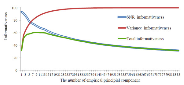
Figure 3 shows the definition of the number of empirical principal components for calculating the complex index of the system, described by 85 statistical indicators. The maximum information content of the system γ = 60.52% is achieved, if nine EPCs are used for calculating the complex index of the system. If we use more EPCs to calculate the complex index, then the information content and the reliability of the computed characteristics is reduced.

Figure 3. Determination of the number of empirical principal components for calculating the complex index of the system.

DownLoad: Full-Size Img PowerPoint

3. Investigation of the quality of integrated indicators

According to the proposed algorithm, the complex indexes of quality of life for Russia's constituent entities for 2007–2016 are calculated. It is worth noting that the determined weighting factors characterize the structure of the system. Over the observed time interval, the structure should be constant. In Russia, there are changes in different areas, so a longer period should not be considered. Data for 2016 was the latest available at the time of this writing.

Variables from (Isakin, 2006) were used for the study (Table 2). All values of the variables are taken from the open directories of Rosstat. Among the listed variables, variables 1, 2, 5, 7, 9, 10, 12, 21, 22, 23 are related to the calculated characteristic by the monotonic increasing dependence, when the optimal j-th value is maximum. The remaining indicators, except for variable 27, the optimal index value is minimal. For variable 27 "net migration" x_j^opt value equals sample mean.

Table 2. Weights of the variables of the first, second and third blocks.

Variable number	Variable Name	Variable weight
	Block 1: Population's welfare
1	Per capita GDP–living wage ratio, units	0.070
2	Per capita income purchasing power relative to living wage, %	0.780
3	Share of people with incomes below living wage, %	0.850
4	The ratio of average income of the richest 20% to the poorest 20% (R\P 20)	−0.430
5	Number of cars per 1 000 people	1.730
6	Share of families on waiting lists for housing, %	1.000
7	Total area of housing resources per resident (m2/10 people)	1.330
8	Share of dilapidated housing, %	0.420
9	Public road density (km/10,000 km2)	0.530
	Block 2: Population quality
10	Life expectancy at birth, years	1.402
11	Mortality rate, infant (per 1,000 live births)	0.166
12	Population growth rate, per 1,000 people	0.667
13	Deaths caused by communicable, parasitic diseases and TB per 100,000 people	1.675
14	Deaths caused by neoplasms per 100,000 people	0.485
15	Deaths caused by cardiovascular diseases per 100,000 people	0.474
16	Deaths caused by respiratory diseases per 100,000 people	1.097
17	Deaths caused by digestive system diseases per 100,000 people	0.842
18	Incidence of injuries, intoxication and other external causes per 100,000 people	1.240
19	Number of disabled people per 1,000 people	0.000
20	Incidence of congenital anomalies per 1,000 people	0.381
21	Specialists with higher education employed in economy, %	1.344
22	Labor force productivity (GRP per average annual number of employed in n economy, thousand rubles/person)	−0.406
23	Graduates from higher and vocational educational institutions per 1,000 people	0.048
	Block 3: Social quality
24	Unemployment, %	0.189
25	Employers engaged in harmful and hazardous working conditions in the average annual number of employed in economy, %	0.467
26	Number of employees injured at work resulting in death or loss of earning capacity for 1 or more days per 1,000employees	1.030
27	Net migration per 10,000 people	0.136
28	Intentional homicides per 100,000 people	0.980
29	Incidence of intentional infliction of grievous bodily harm per 100,000 people	0.933
30	Incidence of rape per 100,000 people	0.955
31	Incidence of robbery and theft per 100,000 people	0.833
32	Incidence of larceny or embezzlement per 100,000 people	0.486
33	Number of registered with drug and substance abuse per 100,000 people	0.761
34	Number of registered with alcohol abuse per 100,000 people	0.811
35	Number of infected with TB per 100,000 people	0.806
36	Mortality from external causes per 100,000 people	0.000
37	Number of people with mental disorders per 100,000 people	0.861

| Show Table

DownLoad: CSV

To obtain the weights of the second block, ten empirical EPСs were used. Used indicators and the resulting weight vectors for these blocks are presented in Table 2.

The number of EPCs for calculating the composite index should maximize the informational value of the obtained solution, defined by (7)—Table 3.

Table 3. Determination of informativeness value of the complex index of Blok 2: Population quality.

	Number of EPCs
	1	2	3	4	5	6	7	8	9	10	11	12	13	14
SNR informativeness	0.98	0.95	0.33	0.33	0.23	0.37	0.38	0.27	0.20	0.26	0.25	0.38	0.28	0.16
Variance informativeness	0.32	0.53	0.63	0.71	0.78	0.84	0.88	0.92	0.95	0.97	0.98	0.99	1.00	1.00
Total informativeness	0.31	0.51	0.58	0.63	0.67	0.70	0.72	0.728	0.729	*0.730*	0.726	0.72	0.70	0.69

| Show Table

DownLoad: CSV

Once the three intermediate composite indices had been constructed, they were agammaegated by allocating a weight to each one of them equal to the proportion to the SNR-informativeness (to the signal level). The block weights are defined in Table 4.

Table 4. Block weights, determined by the SNR-informativeness.

Block	1	2	3
Sum of significant SNRs	172.2	348.1	251.7
Block's weight	0.243	0.464	0.294

| Show Table

DownLoad: CSV

The results are shown in Table 5. The values of the complex indexes obtained vary from 1 to 100 (in 2007). The Republic of Tyva has the minimum unit value; Ingushetia has the maximum value of 100.

Table 5. The complex indexes of quality of life and ratings for Russia's constituent entities for 2007–2016.

Region of the RF	Complex index
Region of the RF	2007	2008	2009	2010	2011	2012	2013	2014	2015	2016
Belgorod reg.	73.6	76.8	80.8	83.2	85.1	85.8	87.3	87.3	90.4	91.6
Bryansk reg.	46.0	47.7	53.0	55.3	59.6	62.2	63.5	65.2	68.0	71.1
Vladimir reg..	44.9	51.2	55.8	59.0	61.3	64.2	65.7	63.6	65.7	69.2
Voronezh reg.	61.3	62.1	64.2	67.3	72.8	77.2	78.3	80.9	83.8	85.7
Ivanovo reg.	37.2	43.1	46.4	47.0	52.8	55.8	59.3	60.8	69.9	72.9
Kaluga reg.	52.2	55.3	59.2	62.0	68.0	70.3	71.8	74.2	75.0	78.5
Kostroma reg.	50.0	51.7	55.7	58.5	60.6	67.1	70.4	72.2	73.0	74.8
Kursk reg.	50.5	54.3	59.2	64.1	65.7	70.5	73.9	74.2	79.5	81.2
Lipetsk reg.	62.0	60.5	65.7	69.5	74.2	75.1	78.5	82.5	82.3	85.4
Moscow reg.	61.6	67.4	72.9	77.4	82.2	84.8	86.9	89.1	93.8	96.0
Oryol reg.	53.8	59.0	61.6	62.8	69.2	70.5	73.0	73.4	75.5	77.9
Ryazan reg.	53.7	59.2	63.7	66.2	71.3	73.4	77.3	76.8	79.3	78.0
Smolensk reg.	39.1	44.4	46.9	51.7	58.9	61.9	66.8	69.3	70.7	73.7
Tambov reg.	54.4	58.0	61.6	64.3	67.8	69.2	74.4	73.3	78.0	81.5
Tver reg.	34.6	38.0	42.9	45.9	53.2	58.8	63.5	63.6	63.6	66.5
Tula reg.	38.7	44.2	51.3	56.7	63.0	64.5	64.4	67.8	69.4	72.9
Yaroslavl reg.	49.5	55.3	60.3	62.5	67.5	68.1	70.0	76.8	75.2	79.4
Moscow	94.6	94.7	98.4	100.9	104.3	104.7	106.9	102.9	105.5	104.7
Rep. of Karelia	44.0	48.0	52.5	53.5	60.6	63.7	68.9	67.6	67.4	71.7
Rep. of Komi	48.0	50.9	53.5	55.9	61.5	64.8	68.9	70.0	70.4	69.7
Arkhangelsk reg.	50.9	54.5	59.7	61.2	65.0	70.0	70.9	72.9	71.3	74.6
Nenets Aut. Okrug	40.0	49.2	52.8	53.2	60.0	66.7	63.1	73.9	73.7	80.4
Vologda reg.	49.2	50.2	52.4	52.8	59.5	64.5	68.8	73.0	74.6	76.7
Kaliningrad reg.	52.5	53.0	58.5	65.1	72.4	77.3	77.9	75.7	79.0	83.6
Leningrad reg..	41.0	46.5	54.3	58.9	64.4	68.0	68.9	69.9	72.3	75.1
Murmansk reg.	68.0	68.7	73.7	77.2	78.6	81.4	86.2	82.9	84.0	86.9
Novgorod reg.	30.8	32.0	38.6	41.4	47.8	54.4	56.0	58.3	58.0	61.7
Pskov reg.	40.8	39.1	43.8	46.4	53.6	57.0	62.9	68.1	66.8	69.7
Saint Petersburg	70.4	73.2	78.8	83.9	87.8	91.1	93.9	91.4	92.0	94.3
Rep. of Adygeya	57.9	60.9	66.2	69.8	72.3	76.7	79.4	81.1	79.9	82.2
Rep. of Kalmykia	58.7	64.0	69.0	64.9	72.2	75.4	78.0	79.8	79.8	83.0
Crimea	-	-	-	-	-	-	-	33.4	34.1	33.8
Krasnodar reg.	65.3	69.0	77.9	75.3	76.4	80.5	85.3	85.5	87.9	91.9
Astrakhan reg.	50.1	53.9	59.2	59.7	65.2	68.7	73.9	75.4	77.9	82.3
Volgograd reg.	58.3	59.9	62.3	64.3	66.9	68.4	71.6	75.7	79.9	85.0
Rostov reg.	60.1	63.0	68.8	69.9	72.0	76.9	79.9	81.2	82.3	83.5
Sevastopol	-	-	-	-	-	-	-	49.8	48.9	48.8
Rep. of Dagestan	82.9	85.0	85.6	88.4	89.4	89.9	91.0	94.2	92.6	98.2
Rep. of Ingushetia	100.0	104.9	99.9	97.6	96.5	96.9	98.1	92.3	94.8	94.6
Kabardino-Balkar Rep.	76.4	82.8	80.6	80.8	82.4	85.4	87.5	86.1	87.9	89.5
Karachay-Cherkessia	69.6	73.2	76.1	79.3	80.6	82.8	86.9	90.2	91.1	96.1
Rep. of North Ossetia	84.9	82.6	82.0	88.5	91.3	93.5	93.4	95.9	94.6	96.2
Chechen Rep.	87.7	93.0	94.2	94.3	93.0	89.5	94.3	94.0	96.2	98.1
Stavropol reg.	69.3	71.5	73.6	79.3	81.8	85.6	89.9	88.6	93.6	94.6
Rep. of Bashkortostan	63.2	66.4	69.0	69.2	72.7	74.2	76.4	74.1	74.3	77.9
Rep. Mary El	38.6	40.0	46.8	48.8	52.1	56.2	60.2	65.7	66.2	71.2
Rep. Of Mordovia	58.5	62.3	65.3	67.3	69.5	72.2	73.9	76.9	79.8	83.1
Rep. of Tatarstan	67.1	69.4	72.9	75.1	77.7	82.0	84.3	83.7	86.4	90.8
Udmurt Rep.	43.1	47.0	52.0	55.3	59.1	64.9	67.9	63.5	68.5	72.0
Chuvash Rep..	43.8	46.9	50.9	52.4	57.8	61.3	63.1	65.4	67.1	71.2
Perm reg.	35.5	39.3	42.5	45.2	50.0	54.7	59.6	61.5	62.2	64.6
Kirov reg.	44.8	47.6	51.8	54.9	60.0	63.5	66.6	70.8	70.9	74.8
Nizhny Novgorod reg.	46.0	50.6	55.9	59.1	65.4	68.8	72.3	74.2	77.4	82.8
Orenburg reg.	48.1	49.9	54.8	58.1	60.2	62.1	64.2	64.3	68.1	73.9
Penza reg.	61.0	62.8	67.3	70.0	75.2	79.5	79.7	77.8	81.5	83.0
Samara reg.	56.9	56.9	59.1	60.3	64.0	67.4	66.5	72.8	74.2	77.0
Saratov reg.	57.8	61.1	63.6	65.6	68.2	72.0	74.9	77.0	77.9	80.9
Ulyanovsk reg.	53.1	57.5	60.8	60.7	64.6	70.3	69.1	69.3	69.2	71.4
Kurgan reg.	40.6	40.8	45.3	46.5	51.4	53.0	55.4	57.2	55.5	59.4
Sverdlovsk reg..	51.5	53.5	56.4	59.6	61.7	64.5	68.7	70.8	69.7	71.8
Tyumen reg.	59.1	62.6	65.9	68.4	74.0	78.7	69.8	70.1	74.5	78.6
Khanty-Mansiysk. A.O.	71.4	73.5	74.6	75.2	80.7	85.9	87.5	87.7	92.0	96.0
Yamalo-Nenets A.O.	75.6	78.7	83.0	82.1	83.6	86.5	92.2	94.4	93.0	94.3
Chelyabinsk reg.	50.2	52.6	56.9	57.7	60.4	62.5	65.9	64.8	67.5	70.1
Rep. of Altai	39.6	38.6	39.9	43.9	49.9	54.1	53.1	54.9	58.4	67.9
Rep. of Buryatia	38.6	38.5	43.0	47.1	50.1	54.4	61.7	59.4	65.4	70.0
Resp. Tuva	1.0	5.1	8.2	12.0	20.6	20.5	25.6	31.4	29.2	29.2
Resp.Khakassia	45.0	46.4	43.5	50.9	51.9	52.4	58.2	59.0	59.7	63.8
Altai reg.	40.3	44.4	47.6	48.0	50.9	53.1	57.8	57.2	62.4	65.7
Transbaikal reg.	36.2	37.6	41.0	42.9	49.4	52.0	53.8	59.7	56.1	60.9
Krasnoyarsk reg.	48.4	50.4	52.5	54.9	58.8	62.1	63.6	64.5	65.5	68.0
Irkutsk reg.	32.2	33.5	34.0	35.2	38.6	43.0	44.7	46.3	48.8	52.5
Kemerovo reg..	28.0	32.4	34.7	35.7	41.3	45.6	51.2	52.6	50.7	52.2
Novosibirsk reg.	46.0	51.0	56.7	59.6	64.3	66.5	68.7	69.7	70.8	73.1
Omsk reg.	46.8	52.2	55.9	59.7	65.6	66.8	64.8	64.6	64.1	70.1
Tomsk reg.	59.1	58.8	60.1	63.4	68.2	71.8	74.0	72.8	74.6	75.3
Yakutia	62.3	58.2	60.4	62.0	65.5	70.5	75.3	79.1	78.4	80.2
Kamchatka Krai	57.1	61.0	64.7	64.1	66.0	71.2	75.6	76.1	78.0	77.6
Primorsky Krai	34.6	39.0	45.3	48.4	50.5	56.4	59.8	63.4	64.0	68.6
Khabarovsk reg.	37.3	40.3	46.6	50.3	53.4	60.1	64.2	63.4	66.6	69.2
Amur reg.	34.5	32.2	33.8	36.8	39.3	46.9	55.5	60.6	60.1	63.0
Magadan reg.	35.7	32.6	44.3	49.1	57.4	57.9	65.6	66.4	70.6	72.8
Sakhalin reg.	34.7	36.4	38.2	42.3	46.6	50.1	56.6	59.5	57.6	61.3
Jewish Authon. reg.	16.6	20.9	24.9	23.9	25.7	33.1	37.6	37.5	36.3	37.8
Chukchi Aut.county	29.9	34.5	30.4	30.9	44.1	45.7	43.0	48.1	52.1	49.6

| Show Table

DownLoad: CSV

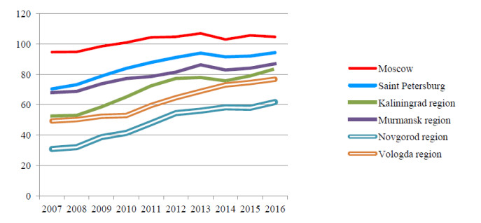
The change in the quality of life for some of Russia's constituent entities is shown in Figure 4. It is interesting to trace the reflection of recent political events on the values of the computed composite index. The impact of the events of 2014 most affected the quality of life in the maritime regions—Kaliningrad and Murmansk—and the financial capitals of Moscow and St. Petersburg. In other regions, the quality of life index is less subject to fluctuations when the political situation changes. Nevertheless, the gap in the quality of life with the leaders is almost not reduced.

Figure 4. The change in the quality of life for some of Russia's constituent entities for 2007–2016.

DownLoad: Full-Size Img PowerPoint

Consistently, the highest complex indices of quality of life for the entire observation period are shown by the constituent entities of the North Caucasus Federal District. Of the 37 indicators, when calculating the complex indices of quality of life, 20 reflect the human physiological well-being and explain (along with the characteristics of national statistics) high indicators for the national republics of the North Caucasus (North Ossetia, Ingushetia, Chechnya, Dagestan, etc.). In these constituent entities of the Russian Federation, it is less likely to get sick, die and undergo criminal violence. The population of these entities is not excessively involved in industry. Life expectancy in Ingushetia is the highest in Russia and exceeds the Novgorod region by 10 years.

4. Estimating the stability of a composite index

Researchers from Russia who compute integrated indicators for different observations complete their research at the stage of calculating and analyzing the ratings obtained, without analyzing the quality problems of the results, in particular robustness and sensitivity (Ajvazjan, 2003; Ajvazjan et al., 2009; Gajdamak and Hohlov, 2009)

The main area of application of composite indexes is the rating of objects. It is the position of the object relative to other objects that is the basis for attracting public attention, and for making political decisions. If small changes in the input data (values of scores or weights) when calculating the composite index fundamentally change the ranking of objects made on the basis of the calculated complex indices, then such an integral indicator cannot be considered reliable. A necessary attribute of the reliability of a composite index is stability relative to perturbations of the original data. In particular, the consequence of this is a slight (on average) change in the rating of objects for different times.

The researchers, who calculate the complex indices for various observations, complete their research at the stage of calculating and analyzing the obtained ratings without analyzing the problems of the quality of the results, in particular, robustness and sensitivity.

It should be noted that the ranks of the 25 member countries of the European Union for 2009–2011, based on the values of the HDI (when calculating the value of the HDI by linear convolution with equal weights) give an average change in the rating for the year of 7.7% (Human Development Reports, 1990–2014). The change in the ratings of more than 15% makes up 14% of cases; more than 30% is 2% of cases. In other words, values are typical in the case of linear convolution with constant weights.

In a study that determines complex indexes of quality of life for the Russian Federation according to the methodology proposed by (Ajvazjan, 2003), ratings for constituent entities were exhibited according to two methods: the weights of the indicators for each year in the linear convolution were determined in one case by experts, in the other by the method proposed by the author. Cases when the rating change amounted to more than 15% are the following: 18 in the case of expert weights, one in the case of calculated weights. The average change in the rating for the first method is 3.6%, for the second method it is 1.6%. Hence, the proposed methodology showed a brilliant quality of the constructed composite index.

However, with careful application of this technique by other authors, the results turn out to be quite different. For example, in the paper (Gajdamak and Hohlov, 2009) the complex indices of the quality of life for municipal formations of the Tyumen region (2005–2008) were calculated. In this case, a change in the rating of more than 15% of the maximum is 48.9% of the total number of cases. In 17.9% of cases, this value exceeds 30%. The average rating change is 16.9%. In the paper (Ajvazjan et al., 2009) values of ratings for municipal formations of the Samara area, calculated by the same method, are given. 45% of objects significantly changed their position in the rating (by 15% or more from the maximum possible rating change). In 21.6% of cases the rating change exceeds 30%. The average rating change is 16.9%.

If small changes in input data while calculating the composite index dramatically change the ranking of objects, then such a composite index cannot be considered reliable. A necessary attribute to the reliability of a composite index is stability relative to perturbations of the original data. In particular, the consequence of this is a slight (on average) change in the rating of objects for different measurements. Schemes for determining weights using factor analysis or the principal component analysis do not have this property.

Let R_t = (r_t1, r_t2, …, r_tm)—the ratings of m objects for the moment t. Known values of the rating sets R_t, R_t+1,..., R_T for the moments t, t + 1, ..., T. R_t—can be considered as a random value uniformly distributed on the interval [1, m]. Numerical characteristics R_t correspond to the numerical characteristics of uniform distribution.

Values of ratings for object i at successive instants of time r_ti, r_{t+1, i}, r_{t+2, i} represent a numerical implementation of a complex functional dependence, a formal description of which is not possible. Changes in ratings over time are dictated mainly by this dependence and to a lesser extent by random factors. The degree of linear connection between the sets of R_t, R_t+1 ratings is high, the Pearson and Spearman correlation coefficients are close to one and do not allow the making of unambiguous conclusions about the quality of the ratings. We propose a method for estimating the stability of a composite index.

If the random variables R_t, R_t+1 are independent, then the variance of the difference of independent random variables is equal to the sum of the variances $D({\Delta _t}){\kern 1pt} = {\kern 1pt} D({R_{t + 1}}{\kern 1pt} - {R_t}){\kern 1pt} \, = {\kern 1pt} D({R_{t + 1}}){\kern 1pt} + {\kern 1pt} D({R_t})\, .$

Because X is even distribution on [a, b], then the variance D(X) = (b-a)²/12. Therefore, D(R_t) = D(R_t+1) = (m-1)²/12 and

$D({\Delta _t}){\kern 1pt} = {\kern 1pt} D({R_{t + 1}}{\kern 1pt} - {R_t}){\kern 1pt} \, = {\kern 1pt} D({R_{t + 1}}){\kern 1pt} + {\kern 1pt} D({R_t}) = \frac{{{{(m - 1)}^2}}}{6}.$

(9)

It is possible to estimate the stability of the complex indexes by estimating the randomness of the difference in the exposed ratings of R_t. Such an estimate of randomness is the fraction of the variance of the realization of the quantity R_t with respect to the variance (9), which reaches a maximum if the ratings R_t, R_t+1 for two consecutive moments of time are absolutely independent of each other and are completely random. Since randomness is not the main reason for rating change, this share should be small.

Table 6 shows the results of assessing the quality of different complex indexes. As a conditional unit of sustainability, we can consider an estimate of the integral index of the HDI, which is about 7% of the possible randomness.

Table 6. Comparison of quality indicators of complex indexes.

Complex index	Source	Period	Weights, source	Number		Evaluation
Complex index	Source	Period	Weights, source	Variables, n	Objects, m	Evaluation
HDI of the EU countries	Human Development Reports, 1990–2014	2009–2011	expert	5	25	6.9
Quality of life of the Russian Federation	Ajvazjan, 2003	1997, 1999	expert	9	79	6.3
Quality of life of the Russian Federation	Ajvazjan, 2003	1997, 2000	expert	9	79	1.2
Quality of life in the Samara Region	Ajvazjan et al., 2009	2002–2004	PCA	11	37	31.5
Quality of Life of the Tyumen Region	Gajdamak and Hohlov, 2009	2005–2008	PCA	17	26	22.7
Quality of life of the Russian Federation	Zhgun, 2017a	2007–2014	PCA	37	83	1.7
Quality of life of the Russian Federation	(*)	2007–2016	PCA	37	85	1.6
SSI. Human Wellbeing	http://www.ssfindex.com/data-all-countries/	2006–2016	expert	9	154	1
SSI. Environmental Wellbeing	http://www.ssfindex.com/data-all-countries/	2006–2016	expert	8	154	3.5
SSI. Economic Wellbeing	http://www.ssfindex.com/data-all-countries/	2006–2016	expert	5	154	4.5
Note: Integral indicators (*) are calculated by the author's method in this paper.

| Show Table

DownLoad: CSV

The magnitude of the estimate, comparable to this value, will indicate a relatively good stability of the integral indicator with respect to the input data. Values that significantly exceed this value characterize the instability of the complex indexes and, consequently, it's of poor quality. In the table below, these are studies Gajdamak and Hohlov (2009) and (Ajvazjan et al., 2009), where the method Ajvazjan (2003) is implemented. The author's method shows good stability.

5. Conclusion

In this paper we consider a solution to the problem of constructing latent complex indexes for the change of a systems quality on the basis of registered measurements for a number of observations in the absence of training. An analysis of the stability of such a solution is provided.

The construction of a system's complex indexes can be considered as a task of extracting the useful signal from a background noise. The signal in this case is the weights of the linear convolution of the indicators. Determined weights should reflect the structure of the system being evaluated. Successful application of the PCA to describe the structure of various system types suggests that the method will also give adequate results for describing social systems. However, the principal component method and factor analysis (even with fixed methods for extracting factors and the method of rotation) determine the structure of the principal components and the main factors for different observations differently. Hence, the method of determining weights using multidimensional analysis cannot be used to compare the characteristics of objects in dynamics.

The reason for this may be the presence of irremovable errors in the data used. Even a small perturbation in the source data can cause a significant change in the weights when using multidimensional analysis methods. As a way out of this situation, a modification of the principal component method is proposed, taking into account the presence of errors in the data used. The algorithm uses a new approach to choosing the number of principal components, to determine the significant loads of the principal components describing the structure of the system, to determining the weights of the considered subsystems, and to determining the informativeness of the selected principal components based on the signal-to-noise ratio parameter.

The solution of the problem requires a detailed understanding of the influence of the errors in the data used on the calculated characteristics. The consequence of stability is on average a slight change (increment) of the ratings of objects for different measurements. This increment can be a posteriori estimated by a sequence of observations using the proposed dispersion criterion. Estimates of different complex indexes' stability by the variance criterion are given. Complex indexes calculated using the proposed modification of the principal component method, which takes into account the presence of errors in the data used, show good resistance to changes in input data.

Conflict of interest

The author declares no conflict of interest in this paper.

References

[1]	Imbabi MS, Carrigan C, McKenna S (2012) Trends and developments in green cement and concrete technology. Int J Sustain Built Environ 1: 194–216. https://doi:10.1016/J.ijsbe.2013.05.001. doi: 10.1016/J.ijsbe.2013.05.001
[2]	Dunuweera SP, Rajapakse RMG (2018) Cement types, composition, uses and advantages of nanocement, environmental impact on cement production, and possible solutions. Adv Mater Sci 2018: 4158682. https://doi:10.1155/2018/4158682 doi: 10.1155/2018/4158682
[3]	Czigler T, Reiter S, Schulze P, et al. (2020) Laying the foundation for zero-carbon cement. Available from: https://www.mckinsey.com/industries/chemicals/our-insights/laying-the-foundation-for-zero-carbon-cement#.
[4]	Shanks W, Dunant CF, Drewniok MP, et al. (2019) How much cement can we do without? Lessons from cement material flows in the UK. Resour Conserv Recycl 141: 441–454. https://doi:10.1016/J.Resconrec.2018.11.002 doi: 10.1016/J.Resconrec.2018.11.002
[5]	Miller SA, Myers RJ (2019) Environmental impacts of alternative cement binders. Environ Sci Technol 54: 677–686. https://doi:10.1021/acs.est.9b05550 doi: 10.1021/acs.est.9b05550
[6]	United States Environmental Protection Agency (EPA), 2019. Available from: https://www.epa.gov.
[7]	Fennell PS, Davis SJ, Mohammed A (2021) Decarbonizing cement production. Joule 5: 1305–1311. https://doi:10.1016/J.Joule.2021.04.011 doi: 10.1016/J.Joule.2021.04.011
[8]	Ishak SA, Hashim H (2015) Low carbon measures for cement plant—a review. J Clean Prod 103: 260–274. https://doi:10.1016/j.jclepro.2014.11.003 doi: 10.1016/j.jclepro.2014.11.003
[9]	Ahmed AK, Ahmad MI, Yusup Y (2020) Issues, impacts, and mitigations of carbon dioxide emissions in the building sector. Sustainability 12: 7427. https://doi:10.3390/SU12187427. doi: 10.3390/SU12187427
[10]	Klufallah MM, Nuruddin MF, Khamidi MF, et al. (2014) Assessment of carbon emission reduction for buildings projects in Malaysia-A comparative analysis. E3S Web Conf 3: 01016. https://doi:10.1051/E3SCONF/20140301016 doi: 10.1051/E3SCONF/20140301016
[11]	Yoro KO, Daramola MO (2020) CO₂ emission sources, greenhouse gases, and the global warming effect, Advances in Carbon Capture: Methods, Technologies and Applications, Woodhead Publishing, 3–28. https://doi:10.1016/B978-0-12-819657-1.00001-32
[12]	Ahmed M, Bashar I, Alam ST, el al. (2021) An overview of Asian cement industry: Environmental impacts, research methodologies and mitigation measures. Sustain Prod Consum 28: 1018–1039. https://doi:10.1016/j.spc.2021.07.024 doi: 10.1016/j.spc.2021.07.024
[13]	Ishak SA, Hashim H (2015) Low carbon measures for cement plant—a review. J Clean Prod 103: 260–274. https://doi:10.1016/j.jclepro.2014.11.003 doi: 10.1016/j.jclepro.2014.11.003
[14]	World Health Organization (WHO), 2022. Available from: https://www.who.int/health-topics/air-pollution.
[15]	Mensah RA, Shanmugam V, Narayanan S, el al. (2021) Biochar-added cementitious materials—A review on mechanical, thermal, and environmental properties. Sustainability 13: 9336. https://doi:10.3390/su13169336 doi: 10.3390/su13169336
[16]	Tun TZ, Bonnet S, Gheewala SH (2021) Emission reduction pathways for a sustainable cement industry in Myanmar. Sustain Prod Consum 27: 449–461. https://doi:10.1016/j.spc.2021.01.016 doi: 10.1016/j.spc.2021.01.016
[17]	Hasanbeigi A, Morrow W, Masanet E, et al. (2013) Energy efficiency improvement and CO₂ emission reduction opportunities in the cement industry in China. Energy Policy 57: 287–297. https://doi:10.1016/j.enpol.2013.01.053 doi: 10.1016/j.enpol.2013.01.053
[18]	Su TL, Chan DYL, Hung CY, et al. (2013) The status of energy conservation in Taiwan's cement industry. Energy Policy 60: 481–486. https://doi:10.1016/j.enpol.2013.04.002 doi: 10.1016/j.enpol.2013.04.002
[19]	Benhelal E, Zahedi G, Shamsaei E, et al. (2013) Global strategies and potentials to curb CO₂ emissions in cement industry. J Clean Prod 51: 142–161. https://doi:10.1016/j.jclepro.2012.10.049 doi: 10.1016/j.jclepro.2012.10.049
[20]	Wang S, Han X (2012) Sustainable cement production with improved energy efficiency and emerging CO₂ mitigation. ASEC 2: 123–128. https://doi:10.4236/aces.2012.21015. doi: 10.4236/aces.2012.21015
[21]	Schneider M, Romer M, Tschudin M, et al. (2011) Sustainable cement production—present and future. Cem Concr Res 41: 642–650. https://doi:10.1016/j.cemconres.2011.03.019 doi: 10.1016/j.cemconres.2011.03.019
[22]	Patrizio P, Fajardy M, Bui M, et al. (2021) CO₂ mitigation or removal: The optimal uses of biomass in energy system decarbonization. IScience 24: 102765. https://doi:10.1016/J.ISCI.2021.102765. doi: 10.1016/J.ISCI.2021.102765
[23]	Chew, KW, Chia SR, Chia WY, et al. (2021) Abatement of hazardous materials and biomass waste via pyrolysis and co-pyrolysis for environmental sustainability and circular economy. Environ Pollut 278: 116836. https://doi:10.1016/j.envpol.2021.116836 doi: 10.1016/j.envpol.2021.116836
[24]	Kumar A, Kumar K, Kaushik N, et al. (2010) Renewable energy in India: current status and future potentials. Renew Sust Energ Rev 14: 2434–2442. https://doi:10.1016/J.RSER.2010.04.003 doi: 10.1016/J.RSER.2010.04.003
[25]	Jacobson MZ (2014) Effects of biomass burning on climate, accounting for heat and moisture fluxes, black and brown carbon, and cloud absorption effects. J Geophys Res Atmos 119: 8980–9002. https://doi:10.1002/2014JD021861 doi: 10.1002/2014JD021861
[26]	Chen J, Li C, Ristovski Z, et al. (2017) A review of biomass burning: Emissions and impacts on air quality, health and climate in China. Sci Total Environ 579: 1000–1034. https://doi:10.1016/j.scitotenv.2016.11.025 doi: 10.1016/j.scitotenv.2016.11.025
[27]	Palanivelu K, Ramachandran A, Raghavan V (2021) Biochar from biomass waste as a renewable carbon material for climate change mitigation in reducing greenhouse gas emissions—a review. Biomass Convers Biorefin 1: 2247–2267. https://doi:10.1007/s13399-020-00604-5 doi: 10.1007/s13399-020-00604-5
[28]	Thomas BS, Yang J, Mo KH, et al. (2021). Biomass ashes from agricultural wastes as supplementary cementitious materials or aggregate replacement in cement/geopolymer concrete: A comprehensive review. J Build Eng 40: 102332. https://doi:10.1016/j.jobe.2021.102332 doi: 10.1016/j.jobe.2021.102332
[29]	Gunarathne V, Ashiq A, Ramanayaka S, et al. (2019) Biochar from municipal solid waste for resource recovery and pollution remediation. Environ Chem Lett 17: 1225–1235. https://doi:10.1007/S10311-019-00866-0 doi: 10.1007/S10311-019-00866-0
[30]	Liu WJ, Jiang H, Yu HQ (2019) Emerging applications of biochar-based materials for energy storage and conversion. Energy Environ Sci 12: 1751–1779. https://doi:10.1039/C9EE00206E doi: 10.1039/C9EE00206E
[31]	Baidoo I, Sarpong DB, Bolwig S, et al. (2016) Biochar amended soils and crop productivity: A critical and meta-analysis of literature. Int J Sustain Dev 5: 414–432. Available from: www.isdsnet.com/ijds.
[32]	Woolf D, Amonette JE, Street-Perrott FA, et al. (2010). Sustainable biochar to mitigate global climate change. Nat Commun 1: 1–9. https://doi:10.1038/NCOMMS1053 doi: 10.1038/NCOMMS1053
[33]	Pariyar P, Kumari K, Jain MK, et al. (2020) Evaluation of change in biochar properties derived from different feedstock and pyrolysis temperature for environmental and agricultural application. Sci Total Environ 713: 136433. https://doi:10.1016/j.scitotenv.2019.136433 doi: 10.1016/j.scitotenv.2019.136433
[34]	Kim S, Lee Y, Lin KYA, et al. (2020) The valorization of food waste via pyrolysis. J Clean Prod 259: 120816. https://doi:10.1016/J.JCLEPRO.2020.120816 doi: 10.1016/J.JCLEPRO.2020.120816
[35]	Demirbas A, Arin G (2002) An overview of biomass pyrolysis. Energy Source 24: 471–482. https://doi:10.1080/00908310252889979 doi: 10.1080/00908310252889979
[36]	Maschio G, Koufopanos C, Lucchesi A (1992) Pyrolysis, a promising route for biomass utilization. Bioresour Technol (United Kingdom) 42: 219–231. https://doi.org/10.1016/0960-8524(92)90025-S doi: 10.1016/0960-8524(92)90025-S
[37]	Li Y, Xing B, Ding Y, et al. (2020) A critical review of the production and advanced utilization of biochar via selective pyrolysis of lignocellulosic biomass. Bioresour Technol 312: 123614. https://doi:10.1016/J.BIORTECH.2020.123614 doi: 10.1016/J.BIORTECH.2020.123614
[38]	Leng L, Huang H, Li H, et al. (2019) Biochar stability assessment methods: a review. Sci Total Environ 647: 210–222. https://doi: 10.1016/j.scitotenv.2018.07.402 doi: 10.1016/j.scitotenv.2018.07.402
[39]	Leng L, Huang H (2018) An overview of the effect of pyrolysis process parameters on biochar stability. Bioresour Technol 270: 627–642. https://doi:10.1016/j.biortech.2018.09.030 doi: 10.1016/j.biortech.2018.09.030
[40]	Tang J, Zhu, W, Kookana R, et al. (2013) Characteristics of biochar and its application in remediation of contaminated soil. J Biosci Bioeng 116: 653–659. https://doi:10.1016/j.jbiosc.2013.05.035 doi: 10.1016/j.jbiosc.2013.05.035
[41]	Ahmad MR, Chen B, Duan H (2020) Improvement effect of pyrolyzed agro-food biochar on the properties of magnesium phosphate cement. Sci Total Environ 718: 137422. https://doi:10.1016/J.SCITOTENV.2020.137422 doi: 10.1016/J.SCITOTENV.2020.137422
[42]	Bhatia SK, Palai AK, Kumar A, et al. (2021) Trends in renewable energy production employing biomass-based biochar. Bioresour Technol 340: 125644. https://doi:10.1016/J.BIORTECH.2021.125644 doi: 10.1016/J.BIORTECH.2021.125644
[43]	Weber K, Quicker P (2018) Properties of biochar. Fuel 217: 240–261. https://doi:10.1016/j.fuel.2017.12.054 doi: 10.1016/j.fuel.2017.12.054
[44]	Yang S, Wi S, Lee J, et al. (2019) Biochar-red clay composites for energy efficiency as eco-friendly building materials: Thermal and mechanical performance. J Hazard Mater 373: 844–855. https://doi:10.1016/J.JHAZMAT.2019.03.079 doi: 10.1016/J.JHAZMAT.2019.03.079
[45]	Sirico A, Bernardi P, Sciancalepore C et al. (2021) Biochar from wood waste as additive for structural concrete. Constr Build Mater 303: 124500. Available from: https://doi:10.1016/j.conbuildmat.2021.124500 doi: 10.1016/j.conbuildmat.2021.124500
[46]	Turovaara M (2022) The effect of high-ratio biochar replacement in concrete on performance properties: Experimental study of biochar addition to concrete mixture[Master's Thesis]. Luleå University of Technology, Sweden.
[47]	Corwin CH (2008) Laboratory manual for Introductory Chemistry: Concepts and Connections, Pearson Higher Ed.
[48]	Lehmann J, Joseph S (2015) Biochar for Environmental Management: Science, Technology and Implementation, Routledge. https://doi:10.4324/9781849770552
[49]	Brewer C, Chuang VJ, Masiello CA, et al. (2014) New approaches to measuring biochar density and porosity. Biomass Bioenerg 66: 176–185. https://doi:10.1016/j.biombioe.2014.03.059 doi: 10.1016/j.biombioe.2014.03.059
[50]	Gupta S, Kashani A (2021) Utilization of biochar from unwashed peanut shell in cementitious building materials—Effect on early age properties and environmental benefits. Fuel Process Technol 218: 106841. https://doi:10.1016/j.fuproc.2021.106841 doi: 10.1016/j.fuproc.2021.106841
[51]	Blanco-Canqui H (2017) Biochar and soil physical properties. Soil Sci Soc Am J 81: 687–711. https://doi:10.2136/SSSAJ2017.01.0017 doi: 10.2136/SSSAJ2017.01.0017
[52]	Werdin J, Fletcher TD, Rayner JP, et al. (2020) Biochar made from low density wood has greater plant available water than biochar made from high density wood. Sci Total Environ 705: 135856. https://doi:10.1016/J.SCITOTENV.2019.135856 doi: 10.1016/J.SCITOTENV.2019.135856
[53]	Leng L, Xiong Q, Yang L, et al. (2021) An overview on engineering the surface area and porosity of biochar. Sci Total Environ 763: 144204. https://doi:10.1016/j.scitotenv.2020.144204 doi: 10.1016/j.scitotenv.2020.144204
[54]	Muthukrishnan S, Gupta S, Kua HW (2019) Application of rice husk biochar and thermally treated low silica rice husk ash to improve physical properties of cement mortar. Theor Appl Fract Mech 104: 102376. https://doi:10.1016/j.tafmec.2019.102376 doi: 10.1016/j.tafmec.2019.102376
[55]	Gupta S, Kua HW, Dai Pang S (2018) Biochar-mortar composite: Manufacturing, evaluation of physical properties and economic viability. Constr Build Mater 167: 874–889. https://doi:10.1016/j.conbuildmat.2018.02.104 doi: 10.1016/j.conbuildmat.2018.02.104
[56]	Gupta S, Kua HW, Koh HJ (2018) Application of biochar from food and wood waste as green admixture for cement mortar. Sci Total Environ 619: 419–435. https://doi:10.1016/J.scitotenv.2017.11.044 doi: 10.1016/J.scitotenv.2017.11.044
[57]	Wijitkosum S, Jiwnok P (2019) Elemental composition of biochar obtained from agricultural waste for soil amendment and carbon sequestration. App Sci 9: 3980. https://doi:10.3390/app9193980 doi: 10.3390/app9193980
[58]	Liu W, Li K, Xu S (2022) Utilizing bamboo biochar in cement mortar as a bio-modifier to improve the compressive strength and crack-resistance fracture ability. Constr Build Mater 327: 126917. https://doi:10.1016/j.conbuildmat.2022.126917 doi: 10.1016/j.conbuildmat.2022.126917
[59]	Graber ER, Tsechansky L, Gerstl Z, et al. (2012) High surface area biochar negatively impacts herbicide efficacy. Plant Soil 353: 95–106. https://doi:10.1007/s11104-011-1012-7 doi: 10.1007/s11104-011-1012-7
[60]	Peterson SC, Jackson MA, Kim S, et al (2012) Increasing biochar surface area: Optimization of ball milling parameters. Powder Technol 228: 115–120. https://doi:10.1016/J.POWTEC.2012.05.005 doi: 10.1016/J.POWTEC.2012.05.005
[61]	Xu D, Cao J, Li Y, et al. (2019) Effect of pyrolysis temperature on characteristics of biochars derived from different feedstocks: A case study on ammonium adsorption capacity. Waste Manage 87: 652–660. https://doi:10.1016/j.wasman.2019.02.049 doi: 10.1016/j.wasman.2019.02.049
[62]	Wani I, Sharma A, Kushvaha V, et al. (2020). Effect of pH, volatile content, and pyrolysis conditions on surface area and O/C and H/C ratios of biochar: towards understanding performance of biochar using simplified approach. J Hazard Toxic Radioact Waste 24: 04020048. https://doi:10.1061/(asce)hz.2153-5515.0000545 doi: 10.1061/(asce)hz.2153-5515.0000545
[63]	Gao Y, Zhang Y, Li A, et al. (2018) Facile synthesis of high-surface area mesoporous biochar for energy storage via in-situ template strategy. Mater Lett 230: 183–186. https://doi:10.1016/j.matlet.2018.07.106 doi: 10.1016/j.matlet.2018.07.106
[64]	Chia CH, Gong B, Joseph SD, et al. (2012) Imaging of mineral-enriched biochar by FTIR, Raman and SEM–EDX. Vib Spectrosc 62: 248–257. https://doi:10.1016/J.VIBSPEC.2012.06.006 doi: 10.1016/J.VIBSPEC.2012.06.006
[65]	Danish A, Mosaberpanah MA, Salim MU, et al. (2021) Reusing biochar as a filler or cement replacement material in cementitious composites: A review. Constr Build Mater 300: 124295. https://doi.10.1016/j.conbuildmat.2021.124295
[66]	Khiari B, Ghouma I, Ferjani AI, et al. (2020) Kenaf stems: Thermal characterization and conversion for biofuel and biochar production. Fuel 262: 116654. https://doi.10.1016/j.fuel.2019.116654
[67]	Gupta S, Krishnan P, Kashani A, et al. (2020) Application of biochar from coconut and wood waste to reduce shrinkage and improve physical properties of silica fume-cement mortar. Constr Build Mater 262: 120688. https://doi:10.1016/j.conbuildmat.2020.120688 doi: 10.1016/j.conbuildmat.2020.120688
[68]	Elnour AY, Alghyamah AA, Shaikh HM, et al. (2019) Effect of pyrolysis temperature on biochar microstructural evolution, physicochemical characteristics, and its influence on biochar/polypropylene composites. Appl Sci 9: 1149. https://doi.org/10.3390/app9061149. doi: 10.3390/app9061149
[69]	Gupta S, Kua HW, Koh HJ (2018) Application of biochar from food and wood waste as green admixture for cement mortar. Sci Total Environ 619: 419–435. https://doi:10.1016/j.scitotenv.2017.11.044 doi: 10.1016/j.scitotenv.2017.11.044
[70]	Ahmad MR, Chen B, Duan H (2020) Improvement effect of pyrolyzed agro-food biochar on the properties of magnesium phosphate cement. Sci Total Environ 718: 137422. https://doi:10.1016/j.scitotenv.2020.137422 doi: 10.1016/j.scitotenv.2020.137422
[71]	Zeidabadi ZA, Bakhtiari S, Abbaslou H, et al. (2018) Synthesis, characterization and evaluation of biochar from agricultural waste biomass for use in building materials. Constr Build Mater 181: 301–308. https://doi:10.1016/j.conbuildmat.2018.05.271 doi: 10.1016/j.conbuildmat.2018.05.271
[72]	Maljaee H, Madadi R, Paiva H, et al. (2021) Sustainable lightweight mortar using biochar as sand replacement. Eur J Environ Civ Eng 26: 8263–8279. https://doi:10.1080/19648189.2021.2021998 doi: 10.1080/19648189.2021.2021998
[73]	Maljaee H, Paiva H, Madadi R, et al. (2021) Effect of cement partial substitution by waste-based biochar in mortars properties. Constr Build Mater 301: 124074. https://doi:10.1016/j.conbuildmat.2021.124074 doi: 10.1016/j.conbuildmat.2021.124074
[74]	Ahmed MB, Zhou JL, Ngo HH, et al. (2016) Insight into biochar properties and its cost analysis. Biomass Bioenerg 84: 76–86. https://doi:10.1016/j.biombioe.2015.11.002 doi: 10.1016/j.biombioe.2015.11.002
[75]	Li C, Hayashi JI, Sun Y, et al. (2021) Impact of heating rates on the evolution of function groups of the biochar from lignin pyrolysis. J Anal Appl Pyrolysis 155: 105031. https://doi:10.1016/J.JAAP.2021.105031 doi: 10.1016/J.JAAP.2021.105031
[76]	Claoston N, Samsuri AW, Ahmad Husni MH, et al. (2014) Effects of pyrolysis temperature on the physicochemical properties of empty fruit bunch and rice husk biochars. Waste Manag Res 32: 331–339. https://doi:10.1177/0734242X14525822 doi: 10.1177/0734242X14525822
[77]	Zhang Y, Ma Z, Zhang Q, et al. (2017) Comparison of the physicochemical characteristics of bio-char pyrolyzed from moso bamboo and rice husk with different pyrolysis temperatures. BioResources 12: 4652–4669. https://doi:10.15376/BIORES.12.3.4652-4669 doi: 10.15376/BIORES.12.3.4652-4669
[78]	Crombie K, Mašek O, Sohi SP, et al. (2013) The effect of pyrolysis conditions on biochar stability as determined by three methods. Gcb Bioenergy 5: 122–131. https://doi:10.1111/GCBB.12030 doi: 10.1111/GCBB.12030
[79]	He M, Xu Z, Sun Y, et al. (2021) Critical impacts of pyrolysis conditions and activation methods on application-oriented production of wood waste-derived biochar. Bioresource Technol 341: 125811. https://doi:10.1016/J.biortech.2021.125811 doi: 10.1016/J.biortech.2021.125811
[80]	Ye L, Zhang J, Zhao J, et al. (2015) Properties of biochar obtained from pyrolysis of bamboo shoot shell. J Anal Appl Pyrolysis 114: 172–178. https://doi: 10.1016/j.jaap.2015.05.016. doi: 10.1016/j.jaap.2015.05.016
[81]	Liu Z, Fei B, Jiang Z (2014) Combustion characteristics of bamboo-biochars. Bioresource Technol 167: 94–99. https://doi:10.1016/j.biortech.2014.05.023 doi: 10.1016/j.biortech.2014.05.023
[82]	Al-Wabel MI, Al-Omran A, El-Naggar AH, et al. (2013) Pyrolysis temperature induced changes in characteristics and chemical composition of biochar produced from conocarpus wastes. Bioresource Technol 131: 374–379. https://doi.org/10.1016/j.biortech.2012.12.165 doi: 10.1016/j.biortech.2012.12.165
[83]	Akhtar A, Sarmah AK (2018) Novel biochar-concrete composites: Manufacturing, characterization and evaluation of the mechanical properties. Sci Total Environ 616: 408–416. https://doi:10.1016/j.scitotenv.2017.10.319 doi: 10.1016/j.scitotenv.2017.10.319
[84]	Zhao C, Liu X, Chen A, et al. (2020) Characteristics evaluation of bio-char produced by pyrolysis from waste hazelnut shell at various temperatures. Energ Source Part A 1–11. https://doi.org/10.1080/15567036.2020.1754530 doi: 10.1080/15567036.2020.1754530
[85]	Gupta S, Kua HW (2020) Application of rice husk biochar as filler in cenosphere modified mortar: Preparation, characterization and performance under elevated temperature. Constr Build Mater 253: 119083. https://doi:10.1016/j.conbuildmat.2020.119083 doi: 10.1016/j.conbuildmat.2020.119083
[86]	ASTM International (2003) Standard specification for coal fly ash and raw or calcined natural pozzolan for use in concrete. ASTM 619-03.
[87]	Zeidabadi ZA, Bakhtiari S, Abbaslou H, et al. (2018) Synthesis, characterization and evaluation of biochar from agricultural waste biomass for use in building materials. Constr Build Mater 181: 301–308. https://doi:10.1016/j.conbuildmat.2018.05.271 doi: 10.1016/j.conbuildmat.2018.05.271
[88]	ASTM International (2019) Standard specification for coal fly ash and raw or calcined natural pozzolan for use in concrete. ASTM 619-19.
[89]	Jeon J, Kim HI, Park JH, et al. (2021) Evaluation of thermal properties and acetaldehyde adsorption performance of sustainable composites using waste wood and biochar. Environ Res 196: 110910. https://doi:10.1016/j.envres.2021.110910 doi: 10.1016/j.envres.2021.110910
[90]	Ngo T, Khudur LS, Hakeem IG, et al. (2022) Wood biochar enhances the valorisation of the anaerobic digestion of chicken manure. Clean Technol Environ Policy 4: 420–439. https://doi:10.3390/cleantechnol4020026 doi: 10.3390/cleantechnol4020026
[91]	Dixit A, Gupta S, Dai Pang S, et al. (2019) Waste valorisation using biochar for cement replacement and internal curing in ultra-high performance concrete. J Clean Prod 238: 117876. https://doi.org/10.1016/j.jclepro.2019.117876 doi: 10.1016/j.jclepro.2019.117876
[92]	Rehrah D, Bansode RR, Hassan O, et al. (2016) Physico-chemical characterization of biochars from solid municipal waste for use in soil amendment. J Anal Appl Pyrolysis 118: 42–53. https://doi:10.1016/J.JAAP.2015.12.022. doi: 10.1016/J.JAAP.2015.12.022
[93]	Silber A, Levkovitch I, Graber ER (2010) pH-dependent mineral release and surface properties of cornstraw biochar: agronomic implications. Environ Sci Technol 44: 9318–9323. https://doi.org/10.1021/es101283d. doi: 10.1021/es101283d
[94]	Gonzalez J, Sargent P, Ennis C (2021) Sewage treatment sludge biochar activated blast furnace slag as a low carbon binder for soft soil stabilisation. J Clean Prod 311: 127553. https://doi:10.1016/j.jclepro.2021.127553. doi: 10.1016/j.jclepro.2021.127553
[95]	Yuan JH, Xu RK (2011) The amelioration effects of low temperature biochar generated from nine crop residues on an acidic Ultisol. Soil Use Manag 27: 110–115. https://doi:10.1111/j.1475-2743.2010.00317.x doi: 10.1111/j.1475-2743.2010.00317.x
[96]	Cosentino I, Restuccia L, Ferro GA, et al. (2019) Type of materials, pyrolysis conditions, carbon content and size dimensions: The parameters that influence the mechanical properties of biochar cement-based composites. Theor Appl Fract Mech 103: 102261. https://doi:10.1016/j.tafmec.2019.102261. doi: 10.1016/j.tafmec.2019.102261
[97]	Malhotra HL (1956) The effect of temperature on the compressive strength of concrete. Mag Concr Res 8: 85–94. https://doi.org/10.1680/macr.1956.8.23.85 doi: 10.1680/macr.1956.8.23.85
[98]	Khoury GA (1992) Compressive strength of concrete at high temperatures: a reassessment. Mag Concr Res 44: 291–309. https://doi:10.1680/MACR.1992.44.161.291 doi: 10.1680/MACR.1992.44.161.291
[99]	Jang JG, Lee HK (2016) Microstructural densification and CO₂ uptake promoted by the carbonation curing of belite-rich Portland cement. Cem Concr Res 82: 50–57. https://doi:10.1016/j.cemconres.2016.01.001 doi: 10.1016/j.cemconres.2016.01.001
[100]	Han T (2020) Application of peanut biochar as admixture in cement mortar. IOP Conf Ser-Earth Environ Sci 531: 012061. https://doi:10.1088/1755-1315/531/1/012061 doi: 10.1088/1755-1315/531/1/012061
[101]	Gupta S, Kua HW (2018) Effect of water entrainment by pre-soaked biochar particles on strength and permeability of cement mortar. Constr Build Mater 159: 107–125. https://doi:10.1016/j.conbuildmat.2017.10.095 doi: 10.1016/j.conbuildmat.2017.10.095
[102]	Sirico A, Bernardi P, Belletti B, et al. (2020) Mechanical characterization of cement-based materials containing biochar from gasification. Constr Build Mater 246: 118490. https://doi:10.1016/j.conbuildmat.2020.118490 doi: 10.1016/j.conbuildmat.2020.118490
[103]	Wang L, Chen L, Tsang DC, et al. (2020) Biochar as green additives in cement-based composites with carbon dioxide curing. J Clean Prod 258: 120678. https://doi:10.1016/j.jclepro.2020.120678 doi: 10.1016/j.jclepro.2020.120678
[104]	Birchall JD, Howard AJ, Kendall K (1981) Flexural strength and porosity of cements. Nature 289: 388–390. https://doi:10.1038/289388a0 doi: 10.1038/289388a0
[105]	Bowlby LK, Saha GC, Afzal MT (2018) Flexural strength behavior in pultruded GFRP composites reinforced with high specific-surface-area biochar particles synthesized via microwave pyrolysis. Composites Part A-Appl S 110: 190–196. https://doi:10.1016/j.compositesa.2018.05.003 doi: 10.1016/j.compositesa.2018.05.003
[106]	Cosentino I, Restuccia L, Ferro GA (2019) Type of materials, pyrolysis conditions, carbon content and size dimensions: The parameters that influence the mechanical properties of biochar cement-based composites. Theor Appl Fract Mech 103: 102261. https://doi:10.1016/j.tafmec.2019.102261 doi: 10.1016/j.tafmec.2019.102261
[107]	Das O, Kim NK, Kalamkarov AL, et al. (2017). Biochar to the rescue: Balancing the fire performance and mechanical properties of polypropylene composites. Polym Degrad Stab 144: 485–496. https://doi: 10.1016/j.polymdegradstab.2017.09.006 doi: 10.1016/j.polymdegradstab.2017.09.006
[108]	Ahmad S, Tulliani JM, Ferro GA, et al. (2015) Crack path and fracture surface modifications in cement composites. Frat ed Integrita Strutt 9: 34. https://doi:10.3221/igf-esis.34.58 doi: 10.3221/igf-esis.34.58
[109]	Gupta S, Kua HW, Low CY (2018) Use of biochar as carbon sequestering additive in cement mortar. Cem Concr Compos 87: 110–129. https://doi:10.1016/j.cemconcomp.2017.12.009 doi: 10.1016/j.cemconcomp.2017.12.009
[110]	Chen B, Li C, Chen L (2009) Experimental study of mechanical properties of normal-strength concrete exposed to high temperatures at an early age. Fire Saf J 44: 997–1002. https://doi:10.1016/j.firesaf.2009.06.007 doi: 10.1016/j.firesaf.2009.06.007
[111]	Gupta S, Kua HW, Dai Pang S (2020) Effect of biochar on mechanical and permeability properties of concrete exposed to elevated temperature. Constr Build Mater 234: 117338. https://doi:10.1016/j.conbuildmat.2019.117338 doi: 10.1016/j.conbuildmat.2019.117338
[112]	Chen X, Wu S, Zhou J (2013) Influence of porosity on compressive and tensile strength of cement mortar. Constr Build Mater 40: 869–874. https://doi:10.1016/J.CONBUILDMAT.2012.11.072 doi: 10.1016/J.CONBUILDMAT.2012.11.072
[113]	Hossain MM, Karim MR, Hasan M, et al. (2016) Durability of mortar and concrete made up of pozzolans as a partial replacement of cement: A review. Constr Build Mater 116: 128–140. https://doi:10.1016/j.conbuildmat.2016.04.147 doi: 10.1016/j.conbuildmat.2016.04.147
[114]	Gupta S, Muthukrishnan S, Kua HW (2021) Comparing influence of inert biochar and silica rich biochar on cement mortar–Hydration kinetics and durability under chloride and sulfate environment. Constr Build Mater 268: 121142. https://doi:10.1016/j.conbuildmat.2020.121142 doi: 10.1016/j.conbuildmat.2020.121142
[115]	Zanotto F, Sirico A, Merchiori S, et al. (2022) Durability of reinforced concrete containing biochar and recycled polymers. Key Eng Mater 919: 188–196. https://doi.org/10.4028/p-mwn300 doi: 10.4028/p-mwn300
[116]	Cuthbertson D, Berardi U, Briens C, et al. (2019) Biochar from residual biomass as a concrete filler for improved thermal and acoustic properties. Biomass Bioenerg 120: 77–83. https://doi:10.1016/j.biombioe.2018.11.007 doi: 10.1016/j.biombioe.2018.11.007
[117]	Wang L, Chen L, Tsang DC, et al. (2019) The roles of biochar as green admixture for sediment-based construction products. Cem Concr Compos 104: 103348. https://doi:10.1016/j.cemconcomp.2019.103348 doi: 10.1016/j.cemconcomp.2019.103348
[118]	Legan M, Gotvajn AŽ, Zupan K (2022) Potential of biochar use in building materials. J Environ Manage 309: 114704. https://doi:10.1016/j.jenvman.2022.114704 doi: 10.1016/j.jenvman.2022.114704
[119]	Berardi U, Naldi M (2017) The impact of the temperature dependent thermal conductivity of insulating materials on the effective building envelope performance. Energ Buildings 144: 262–275. https://doi:10.1016/j.enbuild.2017.03.052 doi: 10.1016/j.enbuild.2017.03.052
[120]	Tan K, Qin Y, Wang J (2022) Evaluation of the properties and carbon sequestration potential of biochar-modified pervious concrete. Constr Build Mater 314: 125648. https://doi:10.1016/j.conbuildmat.2021.125648 doi: 10.1016/j.conbuildmat.2021.125648
[121]	Gupta S, Kua HW (2017) Factors determining the potential of biochar as a carbon capturing and sequestering construction material: critical review. J Mater Civ Eng 29: 04017086. https://doi:10.1061/(asce)mt.1943-5533.0001924 doi: 10.1061/(asce)mt.1943-5533.0001924
[122]	Maljaee H, Madadi R, Paiva H, et al. (2021) Sustainable lightweight mortar using biochar as sand replacement. Eur J Environ Civ Eng 26: 8263–8279. https://doi.org/10.1080/19648189.2021.2021998 doi: 10.1080/19648189.2021.2021998
[123]	Gupta S, Kua HW (2020) Combination of biochar and silica fume as partial cement replacement in mortar: Performance evaluation under normal and elevated temperature. Waste Biomass Valori 11: 2807–2824. https://doi:10.1007/s12649-018-00573-x. doi: 10.1007/s12649-018-00573-x
[124]	Restuccia L, Ferro GA (2016) Promising low cost carbon-based materials to improve strength and toughness in cement composites. Constr Build Mater 126: 1034–1043. https://doi:10.1016/j.conbuildmat.2016.09.101 doi: 10.1016/j.conbuildmat.2016.09.101
[125]	Mrad R, Chehab, G (2019). Mechanical and microstructure properties of biochar-based mortar: An internal curing agent for PCC. Sustainability 11: 2491. https://doi.org/10.3390/su11092491 doi: 10.3390/su11092491
[126]	Maljaee H, Madadi R, Paiva H, et al. (2021) Incorporation of biochar in cementitious materials: A roadmap of biochar selection. Constr Build Mater 283: 122757. https://doi.org/10.1016/j.conbuildmat.2021.122757 doi: 10.1016/j.conbuildmat.2021.122757
[127]	Restuccia, L, Ferro GA, Suarez-Riera D, et al. (2020). Mechanical characterization of different biochar-based cement composites. Procedia Struct Integr 25: 226–233. https://doi.org/10.1016/j.prostr.2020.04.027 doi: 10.1016/j.prostr.2020.04.027

Reader Comments

Your name:*

Email:*
© 2023 the Author(s), licensee AIMS Press. This is an open access article distributed under the terms of the Creative Commons Attribution License (http://creativecommons.org/licenses/by/4.0)