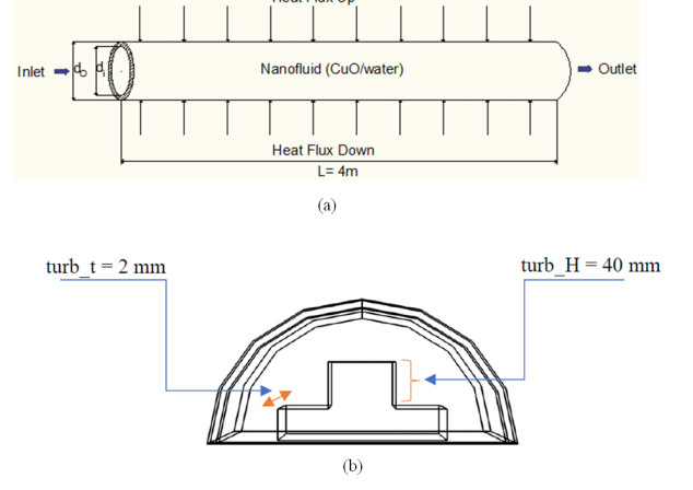
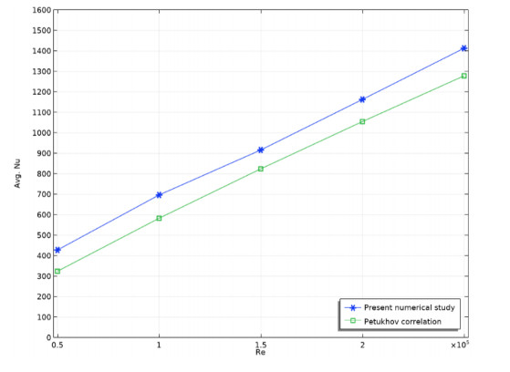
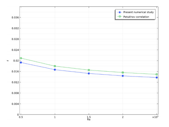
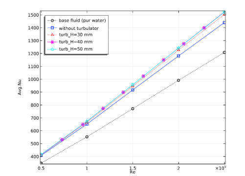
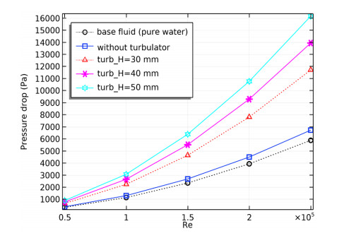
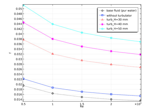
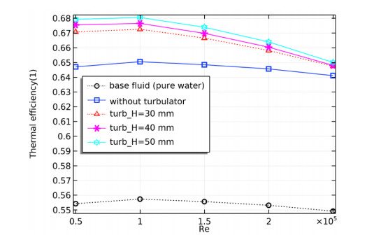
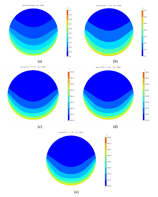
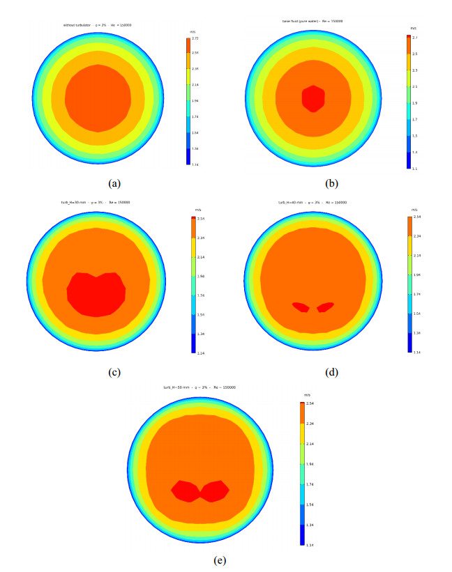
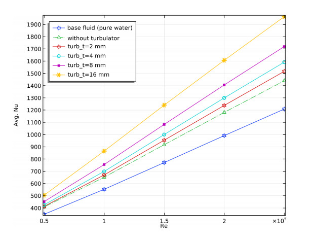
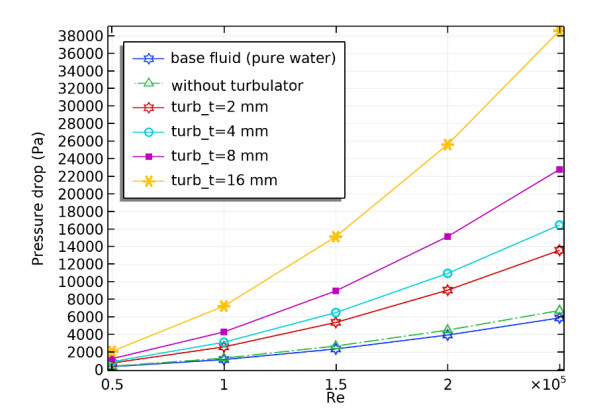
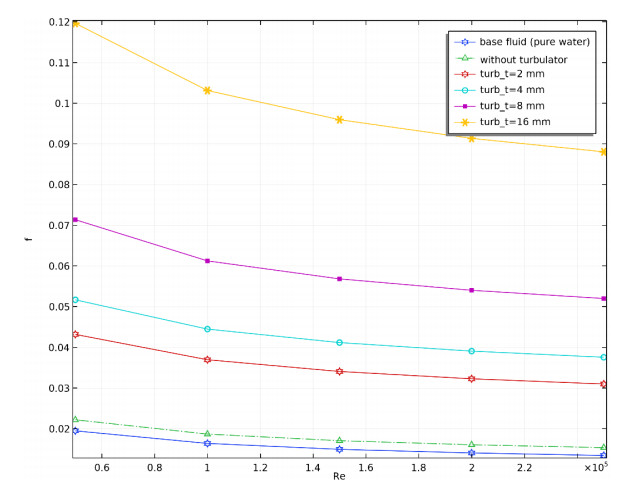
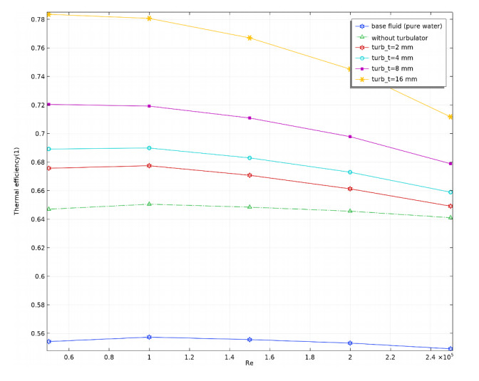
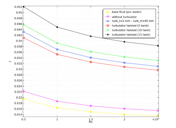
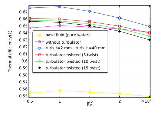
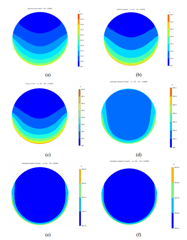
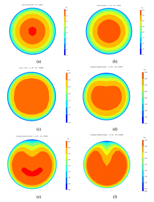
In this study, we numerically investigated the hydrothermal performance of a parabolic trough solar collector system in which nanofluids are used to transfer thermal energy. The single-phase model has been used to evaluate the respective influences of the spherical shape of nanoparticles with a volume fraction of (φ = 3%), Reynolds number varying between 50,000 ≤ Re ≤ 250,000 and the insertion of a turbulator with and without a twisted configuration on the hydrothermal characteristics created by the turbulent forced convection of a CuO/water nanofluid. The shaped turbulator (+) inserted in the absorber tube had a length turb_L = 2.4 m, a height turb_H = 40 mm and a width turb_t = 2 mm. In the second configuration, the considered turbulator was twisted (N_twist = 5, 10 and 15 twists). The turbulator was positioned at 0.6 m from the inlet of the tube and 1 m from the outlet of the collector. The studied performances included the heat transfer characteristics, pressure drop, friction factor, thermal efficiency, temperature and velocity distribution of the outlet field. The most significant contribution of this study is the proposal of the best parameters to increase the thermal and hydraulic efficiency of parabolic troughs by adding a new turbulator with the considered twists.
Citation: Omar Ouabouch, Imad Ait Laasri, Mounir Kriraa, Mohamed Lamsaadi. Investigation of novel turbulator with and without twisted configuration under turbulent forced convection of a CuO/water nanofluid flow inside a parabolic trough solar collector[J]. AIMS Materials Science, 2023, 10(1): 112-138. doi: 10.3934/matersci.2023007
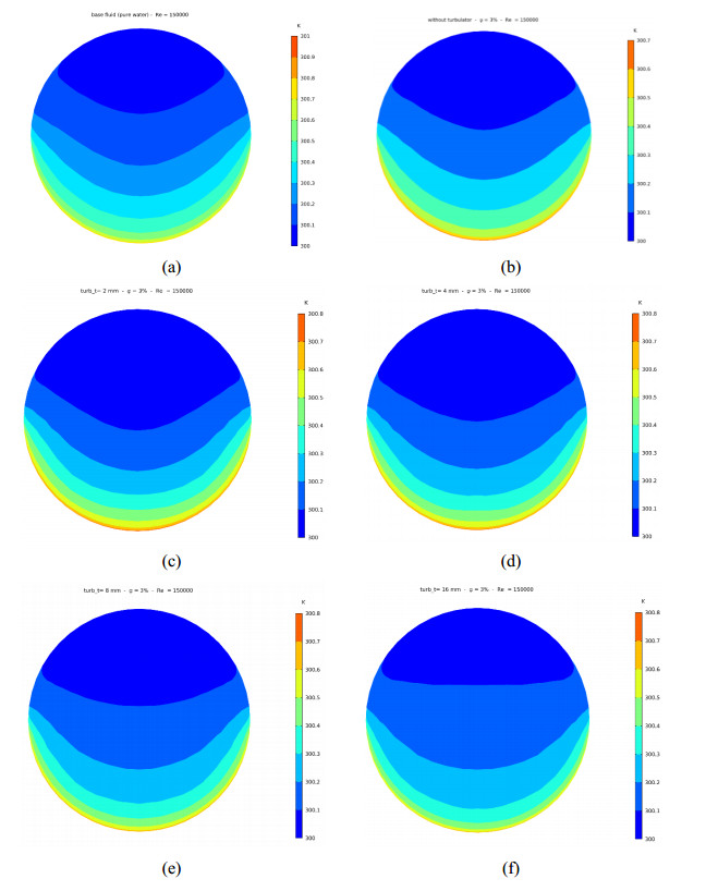
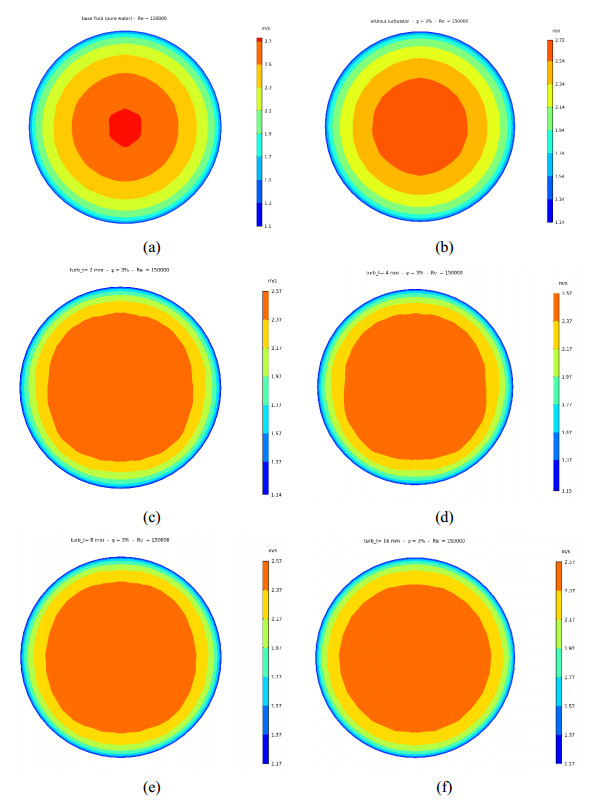
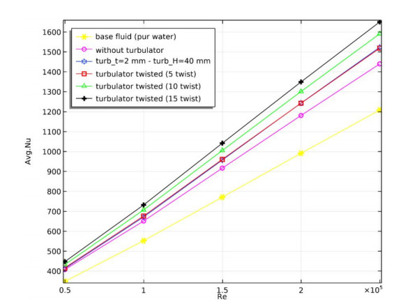
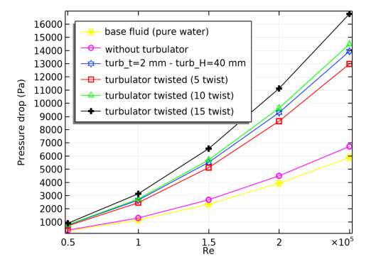
In this study, we numerically investigated the hydrothermal performance of a parabolic trough solar collector system in which nanofluids are used to transfer thermal energy. The single-phase model has been used to evaluate the respective influences of the spherical shape of nanoparticles with a volume fraction of (φ = 3%), Reynolds number varying between 50,000 ≤ Re ≤ 250,000 and the insertion of a turbulator with and without a twisted configuration on the hydrothermal characteristics created by the turbulent forced convection of a CuO/water nanofluid. The shaped turbulator (+) inserted in the absorber tube had a length turb_L = 2.4 m, a height turb_H = 40 mm and a width turb_t = 2 mm. In the second configuration, the considered turbulator was twisted (N_twist = 5, 10 and 15 twists). The turbulator was positioned at 0.6 m from the inlet of the tube and 1 m from the outlet of the collector. The studied performances included the heat transfer characteristics, pressure drop, friction factor, thermal efficiency, temperature and velocity distribution of the outlet field. The most significant contribution of this study is the proposal of the best parameters to increase the thermal and hydraulic efficiency of parabolic troughs by adding a new turbulator with the considered twists.

| [1] |
Shahbaz M, Raghutla C, Chittedi KR, et al. (2020) The effect of renewable energy consumption on economic growth: Evidence from the renewable energy country attractive index. Energy 207: 118162. https://doi.org/10.1016/j.energy.2020.118162 doi: 10.1016/j.energy.2020.118162

|
| [2] |
Bellos E, Tzivanidis C (2019) Alternative designs of parabolic trough solar collectors. Prog Energy Combust Sci 71: 81–117. https://doi.org/10.1016/j.pecs.2018.11.001 doi: 10.1016/j.pecs.2018.11.001
|
| [3] |
Ouabouch O, Laasri IA, Kriraa M, et al. (2022) Effects of flow regime and geometric parameters on the performance of a parabolic trough solar collector using nanofluid. Numer Heat Transf Part A App 82: 1–13. https://doi.org/10.1080/10407782.2022.2078632 doi: 10.1080/10407782.2022.2078632
|
| [4] |
Tembhare SP, Barai DP, Bhanvase BA(2022) Performance evaluation of nanofluids in solar thermal and solar photovoltaic systems: A comprehensive review. Renew Sustain Energy Rev 153: 111738. https://doi.org/10.1016/j.rser.2021.111738 doi: 10.1016/j.rser.2021.111738
|
| [5] |
Qi C, Luo T, Liu M, et al. (2019) Experimental study on the flow and heat transfer characteristics of nanofluids in double-tube heat exchangers based on thermal efficiency assessment. Energy Convers Manag 197: 111877. https://doi.org/10.1016/j.enconman.2019.111877 doi: 10.1016/j.enconman.2019.111877
|
| [6] | Choi SUS, Eastman JA (1995) Enhancing thermal conductivity of fluids with nanoparticles. 1995 International mechanical engineering congress and exhibition, San Francisco, CA (United States. |
| [7] | Ouabouch O, Kriraa M, Lamsaadi M (2021) Stability, thermophsical properties of nanofluids, and applications in solar collectors: A review. 8: 659–684. https://doi.org/10.3934/matersci.2021040 |
| [8] |
Ghasemi SE, Ranjbar AA (2016) Thermal performance analysis of solar parabolic trough collector using nanofluid as working fluid: A CFD modelling study. J Mol Liq 222: 159–166. https://doi.org/10.1016/j.molliq.2016.06.091 doi: 10.1016/j.molliq.2016.06.091
|
| [9] |
Ouabouch O, Laasri IA, Kriraa M, et al. (2021) Modelling and comparison of the thermohydraulic performance with an economical evaluation for a parabolic trough solar collector using different nanofluids. Int J Heat Technol 39: 1763–1769. https://doi.org/10.18280/ijht.390609 doi: 10.18280/ijht.390609
|
| [10] |
Bellos E, Tzivanidis C, Antonopoulos KA, et al. (2016) Thermal enhancement of solar parabolic trough collectors by using nanofluids and converging-diverging absorber tube. Renew Energy 94: 213–222. https://doi.org/10.1016/j.renene.2016.03.062 doi: 10.1016/j.renene.2016.03.062
|
| [11] |
García A, Vicente PG, Viedma A (2005) Experimental study of heat transfer enhancement with wire coil inserts in laminar-transition-turbulent regimes at different Prandtl numbers. Int J Heat Mass Transf 48: 4640–4651. https://doi.org/10.1016/j.ijheatmasstransfer.2005.04.024 doi: 10.1016/j.ijheatmasstransfer.2005.04.024
|
| [12] |
Mwesigye A, Bello-Ochende T, Meyer JP (2015) Multi-objective and thermodynamic optimisation of a parabolic trough receiver with perforated plate inserts. Appl Therm Eng 77: 42–56. https://doi.org/10.1016/j.applthermaleng.2014.12.018 doi: 10.1016/j.applthermaleng.2014.12.018
|
| [13] |
Khan MS, Yan M, Ali HM, et al. (2020) Comparative performance assessment of different absorber tube geometries for parabolic trough solar collector using nanofluid. J Therm Anal Calorim 142: 2227–2241. https://doi.org/10.1007/s10973-020-09590-2 doi: 10.1007/s10973-020-09590-2
|
| [14] |
Liu Y, Chen Q, Hu K, et al. (2016) Flow field optimization for the solar parabolic trough receivers in direct steam generation systems by the variational principle. Int J Heat Mass Transf 102: 1073–1081. https://doi.org/10.1016/j.ijheatmasstransfer.2016.06.083 doi: 10.1016/j.ijheatmasstransfer.2016.06.083
|
| [15] |
Saedodin S, Zaboli M, Ajarostaghi SSM (2021) Hydrothermal analysis of heat transfer and thermal performance characteristics in a parabolic trough solar collector with Turbulence-Inducing elements. Sustain Energy Techn 46: 101266. https://doi.org/10.1016/j.seta.2021.101266 doi: 10.1016/j.seta.2021.101266
|
| [16] |
Olfian H, Ajarostaghi SSM, Farhadi M, et al. (2021) Melting and solidification processes of phase change material in evacuated tube solar collector with U-shaped spirally corrugated tube. Appl Therm Eng 182: 116149. https://doi.org/10.1016/j.applthermaleng.2020.116149 doi: 10.1016/j.applthermaleng.2020.116149
|
| [17] |
Fan F, Qi C, Liu Q, et al. (2020) Effect of twisted turbulator perforated ratio on thermal and hydraulic performance of magnetic nanofluids in a novel thermal exchanger system. Case Stud. Therm Eng 22: 100761. https://doi.org/10.1016/j.csite.2020.100761 doi: 10.1016/j.csite.2020.100761
|
| [18] |
Song X, Dong G, Gao F, et al. (2014) A numerical study of parabolic trough receiver with nonuniform heat flux and helical screw-tape inserts. Energy 77: 771–782. https://doi.org/10.1016/j.energy.2014.09.049 doi: 10.1016/j.energy.2014.09.049
|
| [19] |
Khanafer K, Vafai K (2011) A critical synthesis of thermophysical characteristics of nanofluids. Int J Heat Mass Transf 54: 4410–4428. https://doi.org/10.1016/j.ijheatmasstransfer.2011.04.048 doi: 10.1016/j.ijheatmasstransfer.2011.04.048
|
| [20] |
Xuan Y, Roetzel W (2000) Conceptions for heat transfer correlation of nanofluids. Int J Heat Mass Transf 43: 3701–3707. https://doi.org/10.1016/S0017-9310(99)00369-5 doi: 10.1016/S0017-9310(99)00369-5
|
| [21] |
Brinkman HC (1952) The viscosity of concentrated suspensions and solutions. J Chem Phys 20: 571. https://doi.org/10.1063/1.1700493 doi: 10.1063/1.1700493
|
| [22] | Maxwell JC (1891) A Treatise on Electricity and Magnetism, UK: Clarendon Press. |
| [23] |
Turkyilmazoglu M (2017) Condensation of laminar film over curved vertical walls using single and two-phase nanofluid models. Eur J Mech B/Fluids 65: 184–191. https://doi.org/10.1016/j.euromechflu.2017.04.007 doi: 10.1016/j.euromechflu.2017.04.007
|
| [24] | Yuan SW (1967) Foundations of Fluid Mechanics, New York: Prentice-Hall. |
| [25] |
Chakraborty O, Das B, Gupta R, et al. (2020) Heat transfer enhancement analysis of parabolic trough collector with straight and helical absorber tube. Therm Sci Eng Prog 20: 100718. https://doi.org/10.1016/j.tsep.2020.100718 doi: 10.1016/j.tsep.2020.100718
|
| [26] |
Petukhov BS (2017) Heat transfer and friction in turbulent pipe flow with variable physical properties. Adv Heat Transf 6: 503–564. https://doi.org/10.1016/S0065-2717(08)70153-9 doi: 10.1016/S0065-2717(08)70153-9
|
Figures(24) / Tables(1)

Omar Ouabouch, Imad Ait Laasri, Mounir Kriraa, Mohamed Lamsaadi. Investigation of novel turbulator with and without twisted configuration under turbulent forced convection of a CuO/water nanofluid flow inside a parabolic trough solar collector[J]. AIMS Materials Science, 2023, 10(1): 112-138. doi: 10.3934/matersci.2023007


 DownLoad: