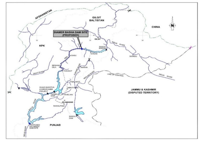
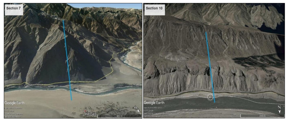
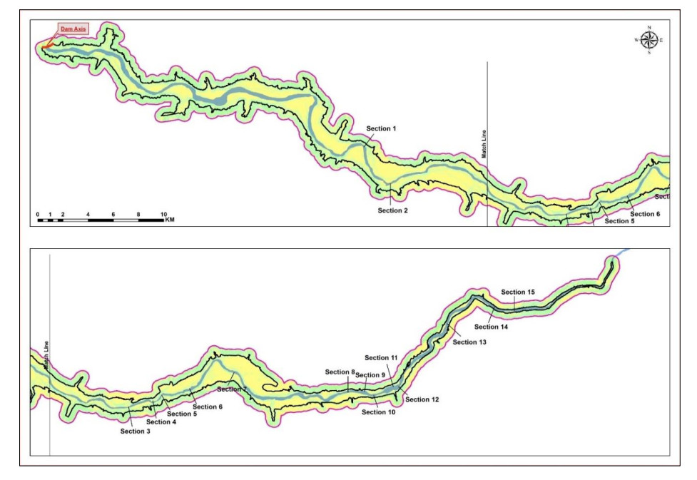
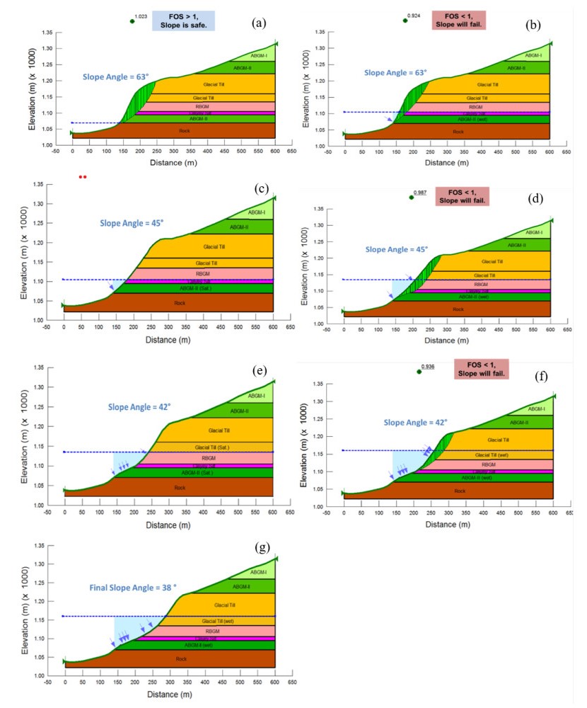
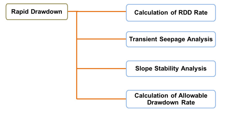
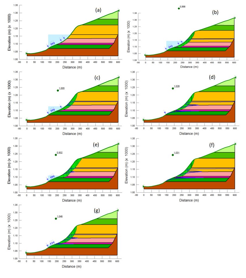
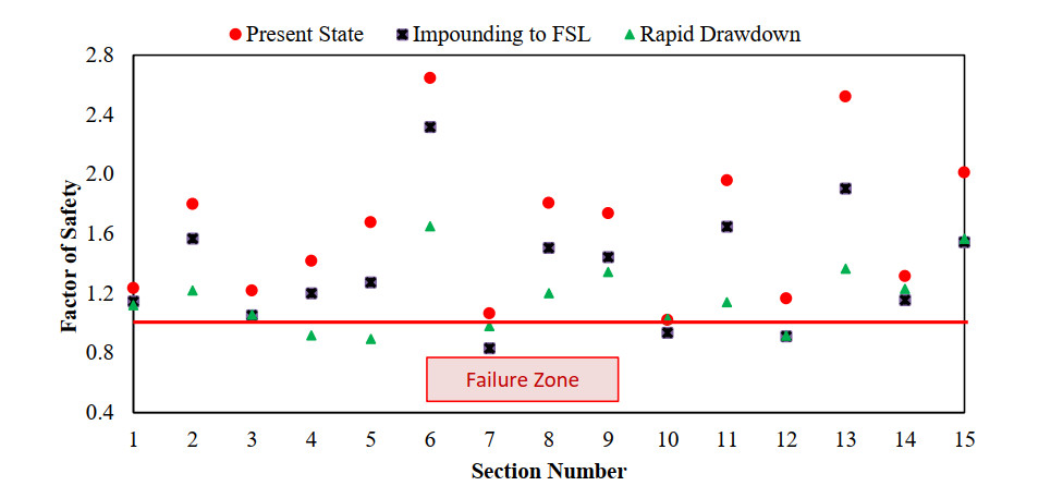
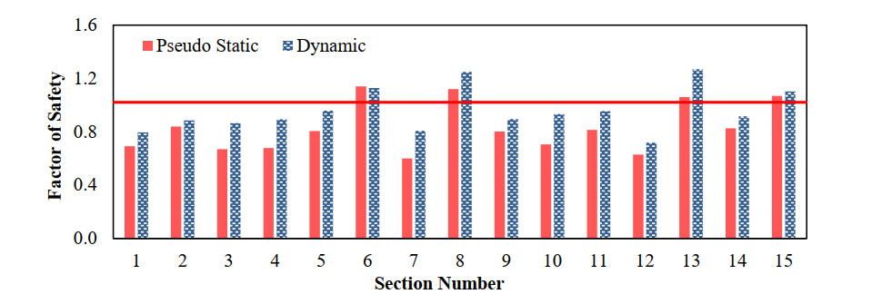
Diamer Basha Dam is an under-construction, 272-meter-high, roller compacted concrete (RCC) dam on the Indus River in Pakistan. Once constructed, it will be the world's highest RCC gravity dam with a 105-kilometer-long reservoir. Most of the reservoir lies in unstable moraine deposits with steep slopes. Events like saturation during reservoir filling, alternate wetting, drawdown during reservoir operation, or a seismic event could trigger a large mass movement of these slopes into the reservoir to disrupt the dam functionality. This work identified the 15 most vulnerable slide areas using digital slope maps, elevation maps, and satellite imagery. Deterministic slope stability analysis was carried out on the identified sections under various stages of reservoir operation for static and seismic loading, using pseudo-static and dynamic analysis approaches. Probabilistic analysis was then performed using Monte Carlo simulation. The findings showed that most moraine deposits would collapse under reservoir filling, rapid drawdown, or seismic activity. Following the assessments, landslide susceptibility maps were generated, and an assessment of potential impacts, including the generation of dynamic waves, reservoir blockage, increased sediment loads, and reduced reservoir storage capacity, was also performed.
Citation: Khalid Ahmad, Umair Ali, Khalid Farooq, Syed Kamran Hussain Shah, Muhammad Umar. Assessing the stability of the reservoir rim in moraine deposits for a mega RCC dam[J]. AIMS Geosciences, 2024, 10(2): 290-311. doi: 10.3934/geosci.2024017
Diamer Basha Dam is an under-construction, 272-meter-high, roller compacted concrete (RCC) dam on the Indus River in Pakistan. Once constructed, it will be the world's highest RCC gravity dam with a 105-kilometer-long reservoir. Most of the reservoir lies in unstable moraine deposits with steep slopes. Events like saturation during reservoir filling, alternate wetting, drawdown during reservoir operation, or a seismic event could trigger a large mass movement of these slopes into the reservoir to disrupt the dam functionality. This work identified the 15 most vulnerable slide areas using digital slope maps, elevation maps, and satellite imagery. Deterministic slope stability analysis was carried out on the identified sections under various stages of reservoir operation for static and seismic loading, using pseudo-static and dynamic analysis approaches. Probabilistic analysis was then performed using Monte Carlo simulation. The findings showed that most moraine deposits would collapse under reservoir filling, rapid drawdown, or seismic activity. Following the assessments, landslide susceptibility maps were generated, and an assessment of potential impacts, including the generation of dynamic waves, reservoir blockage, increased sediment loads, and reduced reservoir storage capacity, was also performed.

| [1] |
Wang L, Wu CZ, Tang LB, et al. (2020) Efficient reliability analysis of earth dam slope stability using extreme gradient boosting method. Acta Geotech 15: 3135-3150. https://doi.org/10.1007/s11440-020-00962-4 doi: 10.1007/s11440-020-00962-4

|
| [2] | Genevois R, Ghirotti M (2005) The 1963 Vaiont Landslide. G di Geol Appl 1: 41-52. |
| [3] |
Babar MS, Israr J, Zhang G, et al. (2022) Analysis of rock slope stability for Mohmand Dam—A comparative study. Cogent Eng 9: 2124939. https://doi.org/10.1080/23311916.2022.2124939 doi: 10.1080/23311916.2022.2124939
|
| [4] |
Mushtaq F, Rehman H, Ali U, et al. (2023) An Investigation of Recharging Groundwater Levels through River Ponding: New Strategy for Water Management in Sutlej River. Sustainability 15: 1047. https://doi.org/10.3390/SU15021047 doi: 10.3390/SU15021047
|
| [5] |
Basharat M, Ali SU, Azhar AH (2014) Spatial variation in irrigation demand and supply across canal commands in Punjab: a real integrated water resources management challenge. Water Policy 16: 397-421. https://doi.org/10.2166/WP.2013.060 doi: 10.2166/WP.2013.060
|
| [6] |
Ali U, Otsubo M, Ebizuka H, et al. (2020) Particle-scale insight into soil arching under trapdoor condition. Soils Found 60: 1171-1188. https://doi.org/10.1016/j.sandf.2020.06.011 doi: 10.1016/j.sandf.2020.06.011
|
| [7] | Otsubo M, Kuwano R, Ali U, et al. (2018) Trapdoor model test and DEM simulation associated with arching. Physical Modelling in Geotechnics, CRC Press, 233-238. |
| [8] | Ali Naqvi U, Otsubo M (2020) A study on arching mechanism in trapdoor model test and equivalent discrete element simulations. 16th Asian Regional Conference on Soil Mechanics and Geotechnical Engineering. |
| [9] |
Wang L, Wu C, Gu X, et al. (2020) Probabilistic stability analysis of earth dam slope under transient seepage using multivariate adaptive regression splines. Bull Eng Geol Environ 79: 2763-2775. https://doi.org/10.1007/s10064-020-01730-0 doi: 10.1007/s10064-020-01730-0
|
| [10] | Santosh S, Khazanchi RN, Mishra A, et al. (2017) Reservoir Rim Stability: A Case Study of Punatsangchhu-I Hydroelectric Project Bhutan. INDOROCK 2017: 7th Indian Rock Conference, New Delhi, India. |
| [11] | MWH Consultants (2013) Preliminary Reservoir Slope Stability Assessment for Susitna-Watana Dam. Available from: https://www.arlis.org/docs/vol1/Susitna2/2/SuWa289/SuWa289sec4-5att3.pdf. |
| [12] |
Wang Y, Liu X, Zhang X, et al. (2023) Dynamic response characteristics of moraine-soil slopes under the combined action of earthquakes and cryogenic freezing. Cold Reg Sci Technol 211: 103854. https://doi.org/10.1016/j.coldregions.2023.103854 doi: 10.1016/j.coldregions.2023.103854
|
| [13] |
Klimeš J, Novotný J, Novotná I, et al. (2016) Landslides in moraines as triggers of glacial lake outburst floods: example from Palcacocha Lake (Cordillera Blanca, Peru). Landslides 13: 1461-1477. https://doi.org/10.1007/s10346-016-0724-4 doi: 10.1007/s10346-016-0724-4
|
| [14] | Ghimire A, Gajurel A (2020) Moraine dam stability analysis of Ngozumpa glacier in Gokyo area, Nepal. American Geophysical Union, Fall Meetin. Available from: https://www.agu.org/fall-meeting-2020. |
| [15] | Anbalagan A, Kumar A (2015) Reservoir induced landslides-a case study of reservoir rimregion of Tehri Dam. TIFAC-IDRiM Conference, New Delhi, India. |
| [16] |
Chen XP, Huang JW (2011) Stability analysis of bank slope under conditions of reservoir impounding and rapid drawdown. J Rock Mech Geotech Eng 3: 429-437. https://doi.org/10.3724/SP.J.1235.2011.00429 doi: 10.3724/SP.J.1235.2011.00429
|
| [17] |
Yin YP, Huang BL, Wang WP, et al. (2016) Reservoir-induced landslides and risk control in Three Gorges Project on Yangtze River, China. J Rock Mech Geotech Eng 8: 577-595. https://doi.org/10.1016/J.JRMGE.2016.08.001 doi: 10.1016/J.JRMGE.2016.08.001
|
| [18] |
Chuaiwate P, Jaritngam S, Panedpojaman P, et al. (2022) Probabilistic Analysis of Slope against Uncertain Soil Parameters. Sustainability 14: 14530. https://doi.org/10.3390/su142114530 doi: 10.3390/su142114530
|
| [19] |
Kumar S, Choudhary SS, Burman A, et al. (2023) Probabilistic Slope Stability Analysis of Mount St. Helens Using Scoops3D and a Hybrid Intelligence Paradigm. Mathematics 11: 3809. https://doi.org/10.3390/math11183809 doi: 10.3390/math11183809
|
| [20] |
Petterson MG (2010) A Review of the geology and tectonics of the Kohistan island arc, north Pakistan. Geol Soc London Spec Publ 338: 287-327. https://doi.org/10.1144/SP338.14 doi: 10.1144/SP338.14
|
| [21] |
Khan SD, Walker DJ, Hall SA, et al. (2009) Did the Kohistan-Ladakh island arc collide first with India? GSA Bull 121: 366-384. https://doi.org/10.1130/B26348.1 doi: 10.1130/B26348.1
|
| [22] |
Ewing TA, Müntener O (2018) The mantle source of island arc magmatism during early subduction: Evidence from Hf isotopes in rutile from the Jijal Complex (Kohistan arc, Pakistan). Lithos 308-309: 262-277. https://doi.org/10.1016/J.LITHOS.2018.03.005 doi: 10.1016/J.LITHOS.2018.03.005
|
| [23] |
Bignold SM, Treloar PJ, Petford N (2006) Changing sources of magma generation beneath intra-oceanic island arcs: An insight from the juvenile Kohistan island arc, Pakistan Himalaya. Chem Geol 233: 46-74. https://doi.org/10.1016/J.CHEMGEO.2006.02.008 doi: 10.1016/J.CHEMGEO.2006.02.008
|
| [24] |
Jagoutz O, Müntener O, Burg JP, et al. (2006) Lower continental crust formation through focused flow in km-scale melt conduits: The zoned ultramafic bodies of the Chilas Complex in the Kohistan island arc (NW Pakistan). Earth Planet Sci Lett 242: 320-342. https://doi.org/10.1016/J.EPSL.2005.12.005 doi: 10.1016/J.EPSL.2005.12.005
|
| [25] |
Dhuime B, Bosch D, Garrido CJ, et al. (2009) Geochemical Architecture of the Lower- to Middle-crustal Section of a Paleo-island Arc (Kohistan Complex, Jijal-Kamila Area, Northern Pakistan): Implications for the Evolution of an Oceanic Subduction Zone. J Petrol 50: 531-569. https://doi.org/10.1093/PETROLOGY/EGP010 doi: 10.1093/PETROLOGY/EGP010
|
| [26] |
Iturrizaga L (2001) Lateroglacial valleys and landforms in the Karakoram Mountains (Pakistan). GeoJournal 54: 397-428. https://doi.org/10.1023/A:1021365416056 doi: 10.1023/A:1021365416056
|
| [27] | GEOSLOPE (2012) User Manual, GEO-SLOPE. GEO-SLOPE International Ltd Calgary, Canada. |
| [28] |
Lebourg T, Riss J, Pirard E (2004) Influence of morphological characteristics of heterogeneous moraine formations on their mechanical behaviour using image and statistical analysis. Eng Geol 73: 37-50. https://doi.org/10.1016/J.ENGGEO.2003.11.004 doi: 10.1016/J.ENGGEO.2003.11.004
|
| [29] | Wang BL, Yao LK, Zhao HX, et al. (2018) The maximum height and attenuation of impulse waves generated by subaerial landslides. Shock Vib 2018.https://doi.org/10.1155/2018/1456579 |
 geosci-10-02-017-s001.pdf geosci-10-02-017-s001.pdf |
 |
Figures(16) / Tables(4)

Khalid Ahmad, Umair Ali, Khalid Farooq, Syed Kamran Hussain Shah, Muhammad Umar. Assessing the stability of the reservoir rim in moraine deposits for a mega RCC dam[J]. AIMS Geosciences, 2024, 10(2): 290-311. doi: 10.3934/geosci.2024017


 DownLoad: