Impact of COVID-19 on tourism sector: a case study of Rajasthan, India

Rajeev Singh Chandel; Shruti Kanga; Suraj Kumar Singh; Rajeev Singh Chandel; Shruti Kanga; Suraj Kumar Singh

doi:10.3934/geosci.2021014

AIMS Geosciences

2021, Volume 7, Issue 2: 224-243. doi: 10.3934/geosci.2021014

Previous Article Next Article

Research article Topical Sections

Impact of COVID-19 on tourism sector: a case study of Rajasthan, India

1.
Centre for Climate Change and Water Research, Suresh Gyan Vihar University, Jaipur, Rajasthan, India
2.
Centre for Sustainable Development, Suresh Gyan Vihar University, Jaipur, Rajasthan, India

Received: 15 April 2021 Accepted: 15 June 2021 Published: 17 June 2021

Background
SARS-CoV-2 or Severe Acute Respiratory Syndrome, is a virus that causes severe respiratory illness, also known as COVID-19, is a global pandemic caused by a novel coronavirus, firstly reported China (Wuhan City) on Dec, 2019. In India, Kerala is the first state in which the COVID-19 first case has registered which has raised to three cases by 3 Feb, 2020.
Purpose
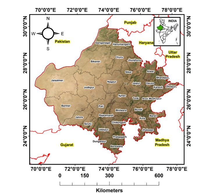
The aim of this research is to map the impact and assessment of the COVID 19 pandemic situation using geospatial technology in Rajasthan and suggest various measures to control the pandemic situation.
Objectives
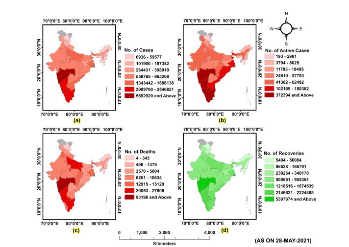
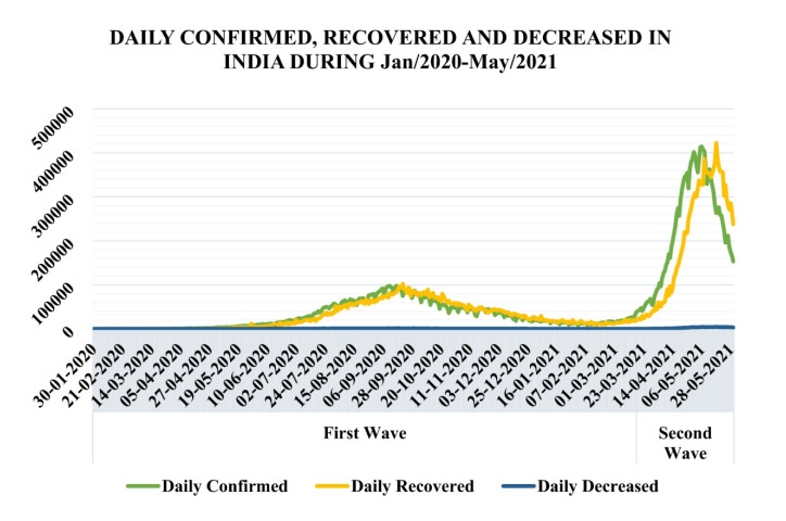
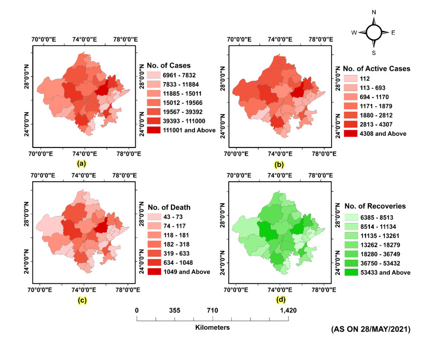
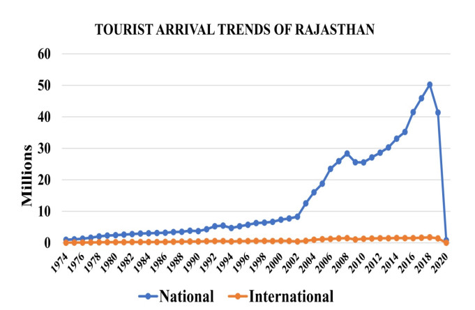
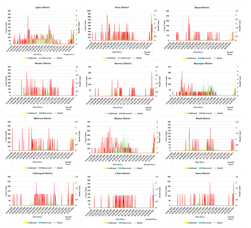
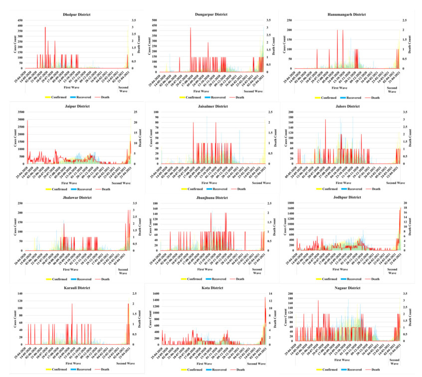
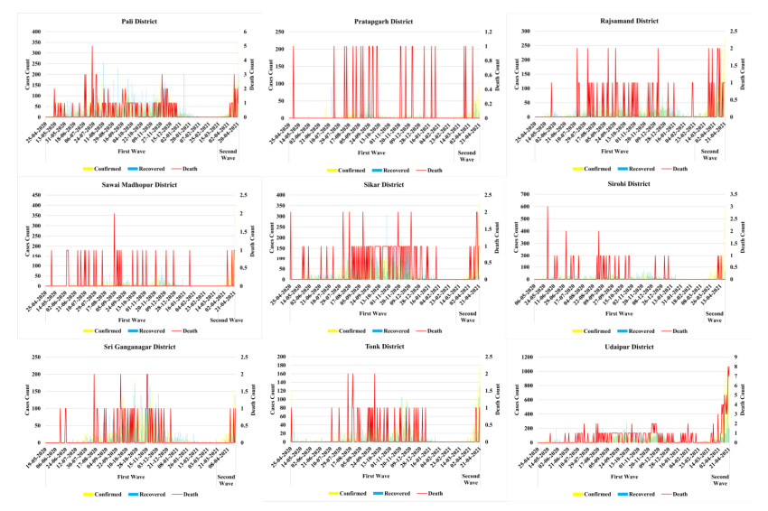
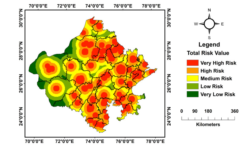
(a) Assessing and mapping the affected parts of Rajasthan and evaluating the risk of the pandemic on tourism, and (b) Initially tracking and forecasting the cases of COVID-19 in the study area.
Methodology
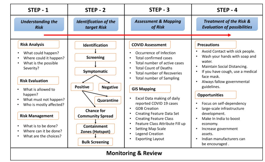
The methodology consists of four main phases. In the first phase understanding the risk of the pandemic situation at three primary levels i.e. risk analysis, risk evaluation, risk management after that, second step is to identify the target risk zones of COVID-19 cases using geospatial technology based on bulk screening. Assessment and mapping of pandemic risk is the third phase. In the fourth phase, treatment of the risk and evaluation of future occurrence possibilities.
Result
COVID 19 pandemic is the greatest threat globally. Geospatial technology provides valuable support in assessing and mapping the risk of COVID 19 cases in Rajasthan at the initial level.
Conclusion
This study shows that the geospatial technique contributes very significantly in detecting pre and post COVID 19 pandemic conditions and helps in proper decision-making, not only in Rajasthan but also in the entire world.
- COVID-19,
- tourism,
- geospatial technology,
- hotspots,
- risk zone mapping
Citation: Rajeev Singh Chandel, Shruti Kanga, Suraj Kumar Singh. Impact of COVID-19 on tourism sector: a case study of Rajasthan, India[J]. AIMS Geosciences, 2021, 7(2): 224-243. doi: 10.3934/geosci.2021014

Related Papers:

Abstract

Background

SARS-CoV-2 or Severe Acute Respiratory Syndrome, is a virus that causes severe respiratory illness, also known as COVID-19, is a global pandemic caused by a novel coronavirus, firstly reported China (Wuhan City) on Dec, 2019. In India, Kerala is the first state in which the COVID-19 first case has registered which has raised to three cases by 3 Feb, 2020.

Purpose

The aim of this research is to map the impact and assessment of the COVID 19 pandemic situation using geospatial technology in Rajasthan and suggest various measures to control the pandemic situation.

Objectives

(a) Assessing and mapping the affected parts of Rajasthan and evaluating the risk of the pandemic on tourism, and (b) Initially tracking and forecasting the cases of COVID-19 in the study area.

Methodology

The methodology consists of four main phases. In the first phase understanding the risk of the pandemic situation at three primary levels i.e. risk analysis, risk evaluation, risk management after that, second step is to identify the target risk zones of COVID-19 cases using geospatial technology based on bulk screening. Assessment and mapping of pandemic risk is the third phase. In the fourth phase, treatment of the risk and evaluation of future occurrence possibilities.

Result

COVID 19 pandemic is the greatest threat globally. Geospatial technology provides valuable support in assessing and mapping the risk of COVID 19 cases in Rajasthan at the initial level.

Conclusion

This study shows that the geospatial technique contributes very significantly in detecting pre and post COVID 19 pandemic conditions and helps in proper decision-making, not only in Rajasthan but also in the entire world.

References

[1]	WHO. Coronavirus, 2020. Available from: https://www.who.int/health-topics/coronavirus#tab=tab_1.
[2]	Kumar J, Sahoo S, Bharti B, et al. (2020) Spatial distribution and impact assessment of COVID-19 on human health using geospatial technologies in India Spatial distribution and impact assessment of COVID-19 on human health using geospatial technologies in India. Int J Multidiscip Res Dev 7: 57–64.
[3]	Choudhary M (2020) Esri creates dashboard to map spread of COVID 19 cases in India - Geospatial World. geoworldmedia. Available from: https://www.geospatialworld.net/blogs/esri-creates-dashboard-to-map-spread-of-covid-19-cases-in-india/.
[4]	Chandel RS, Kanga S (2018) Use of Geospatial Techniques to Manage the Tourists & Administration: A Case Study of Mount Abu, Rajasthan. We Int J Sci Tech 13: 63–78.
[5]	Kanga S, Meraj G, Sudhanshu, et al. (2021) Analyzing the Risk to COVID‐19 Infection using Remote Sensing and GIS. Risk Anal 41: 801–813. doi: 10.1111/risa.13724
[6]	Ranga V, Pani P, Kanga S, et al. (2020) Health GIS - A Long lasting Solution for the Effective Pandemic Management in India. AGU. Available from: https://agu.confex.com/agu/COVIDsymp2020/meetingapp.cgi/Paper/664109.
[7]	MoHFW (2021) Available from: https://www.mohfw.gov.in/.
[8]	Wathore R, Gupta A, Bherwani H, et al. (2020) Understanding air and water borne transmission and survival of coronavirus: Insights and way forward for SARS-CoV-2. Sci Total Environ 749: 141486. doi: 10.1016/j.scitotenv.2020.141486
[9]	Meraj G, Farooq M, Singh SK, et al. (2020) Coronavirus pandemic versus temperature in the context of Indian subcontinent: a preliminary statistical analysis. Environ Dev Sustain 10: 1–11. doi: 10.5296/emsd.v10i1.17820
[10]	The Hindu (2020) Coronavirus India lockdown Day 144 updates. Available from: https://www.thehindu.com/news/national/coronavirus-india-lockdown-august-15-2020-live-updates/article32361213.ece.
[11]	IANS (2021) Rajasthan reports first case of coronavirus. Outlookindia. Available from: https://www.outlookindia.com/newsscroll/rajasthan-reports-first-case-of-coronavirus/1749775.
[12]	Deshmane A (2020) In Rajasthan, The Economic Impact Of Lockdown Could Outweigh The Coronavirus Health Crisis. Huffpost. Available from: https://www.huffingtonpost.in/entry/in-rajasthan-the-economic-impact-of-lockdown-could-outweigh-the-coronavirus-health-crisis_in_5e987da8c5b6ead140094da9.
[13]	Sridharan A (2019) Flying Colors: Analyzing the Impact of Travel and Tourism on People and Their Communities. Plan II Honor Theses-Openly Available.
[14]	Kanga S, Sudhanshu, Meraj G, et al. (2020) Reporting the Management of COVID-19 Threat in India Using Remote Sensing and GIS-Based Approach. Geocarto Int 6049: 1–6. doi: 10.1080/10106049.2020.1778106
[15]	Kanga S, Meraj G, Farooq M, et al. (2021) Risk assessment to curb COVID-19 contagion: A preliminary study using remote sensing and GIS. Available from: https://doi.org/10.21203/rs.3.rs-37862/v1.
[16]	Yang J, Huang F (2011) Research on management of ecotourism based on economic models. Energy Procedia 5: 1563–1567. doi: 10.1016/j.egypro.2011.03.267
[17]	Dash J (2020) Covid-19 impact: Tourism industry to incur Rs 1.25 trn revenue loss in 2020. Bus Stand. Available from: https://www.business-standard.com/article/economy-policy/covid-19-impact-tourism-industry-to-incur-rs-1-25-trn-revenue-loss-in-2020-120042801287_1.html.
[18]	Pulla P (2020) Covid-19: India imposes lockdown for 21 days and cases rise. BMJ 368: m1251.
[19]	Kanga S, Meraj G, Das B, et al. (2020) Modeling the spatial pattern of sediment flow in lower Hugli estuary, West Bengal, India by quantifying suspended sediment concentration (SSC) and depth conditions using geoinformatics. Appl Comput Geosci 8: 100043. doi: 10.1016/j.acags.2020.100043
[20]	Ranasinghe R, Damunupola A, Wijesundara S, et al. (2020) Tourism after Corona: Impacts of Covid 19 Pandemic and Way Forward for Tourism, Hotel and Mice Industry in Sri Lanka. SSRN Electron J.
[21]	Kanga S, Thakur K, Kumar S, et al. (2014) Potential of Geospatial Techniques to Facilitate the Tourist & Administration : A Case Study of Shimla Hill Station, Himachal. Int J Adv Remote Sens GIS 3: 681–698.
[22]	Chandel RS, Kanga S (2020) Sustainable Management of Ecotourism in Western Rajasthan, India: A Geospatial Approach. Geo J Tour Geosites 29: 521–533. doi: 10.30892/gtg.29211-486
[23]	Shekhawat A (2018) Investment Environment in Rajasthan: Trends and Issues. Rajasthan Econ J 42: 1–14.
[24]	Statista (2021) India - tourist arrivals in Kerala by type 2017 Statista. Available from: https://www.statista.com/statistics/1026993/india-tourist-arrivals-in-rajasthan-by-type/.
[25]	Chandel RS, Kanga S (2019) Ecotourism Potential in Western Rajasthan. A Case Study of Jaisalmer District. SGVU J Clim Chang Water 6: 8–15.
[26]	Rodríguez-Antón JM, Alonso-Almeida MDM (2020) COVID-19 impacts and recovery strategies: The case of the hospitality industry in Spain. Sustainability 12: 8599. doi: 10.3390/su12208599
[27]	Aninews. 2,167 positive COVID-19 cases in Haridwar in last five days; Kumbh Mela to continue, 2021. Available from: https://www.aninews.in/news/national/general-news/2167-positive-covid-19-cases-in-haridwar-in-last-five-days-kumbh-mela-to-continue20210415165122/.

Reader Comments

your name:*

Email:*
© 2021 the Author(s), licensee AIMS Press. This is an open access article distributed under the terms of the Creative Commons Attribution License (http://creativecommons.org/licenses/by/4.0)