


Figure 1.
(a) The trivial state steady E0 of system (1.7) is globally asymptotically stable. (b) The positive constant state steady E∗ of system (1.7) is globally asymptotically stable.
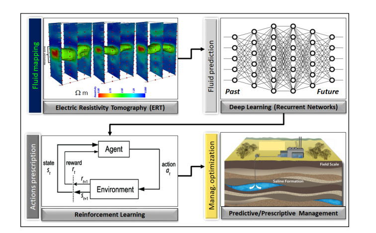
In this paper, I introduce a comprehensive workflow aimed at optimizing oil production and CO2 geological storage. I show that the same methodology can be applied to different categories of problems: a) real-time reservoir fluid mapping for predicting and delaying water breakthrough time as far as possible in oil production; b) real-time CO2 mapping for maximizing the sweep efficiency and storage capacity of CO2 in geological formations. Despite their intrinsic differences, these types of problems share common aspects, issues and possible solutions. In both cases, various geophysical techniques can be applied, including Electric Resistivity Tomography (briefly ERT) for accurate fluid mapping and monitoring. This method is highly effective and sensitive for detecting the type of fluid and for estimating saturation in the geological formations. The robustness and the accuracy of the ERT models increase if densely spaced electrodes layouts are permanently deployed into the production and injection wells. In the first part of the paper, I discuss how in both scenarios of oil production and CO2 storage, we can apply time-lapse borehole ERT method for mapping fluids in the reservoir. Next, I discuss how to apply various techniques of time-series analysis for predicting the evolution of the fluids distribution over time. Finally, using Q-Learning, that is a specific Reinforcement Learning method, I discuss how we can optimize the decisional workflow using our models about past, real-time and predicted fluids displacement. The result is the definition of a "best policy" addressed to both problems of optimized oil production and safe CO2 geological storage. In the second part of the paper, I show benefits and limitations of my approach with the support of synthetic tests.
Citation: Paolo Dell'Aversana. Reservoir prescriptive management combining electric resistivity tomography and machine learning[J]. AIMS Geosciences, 2021, 7(2): 138-161. doi: 10.3934/geosci.2021009
| [1] | Sang Jo Yun, Sangbeom Park, Jin-Woo Park, Jongkyum Kwon . Some identities of degenerate multi-poly-Changhee polynomials and numbers. Electronic Research Archive, 2023, 31(12): 7244-7255. doi: 10.3934/era.2023367 |
| [2] | Weiran Ding, Jiansong Li, Yumeng Jia, Wanru Yang . Tractability of L2-approximation and integration over weighted Korobov spaces of increasing smoothness in the worst case setting. Electronic Research Archive, 2025, 33(2): 1160-1184. doi: 10.3934/era.2025052 |
| [3] | Mohra Zayed, Gamal Hassan . Kronecker product bases and their applications in approximation theory. Electronic Research Archive, 2025, 33(2): 1070-1092. doi: 10.3934/era.2025048 |
| [4] | Muajebah Hidan, Ahmed Bakhet, Hala Abd-Elmageed, Mohamed Abdalla . Matrix-Valued hypergeometric Appell-Type polynomials. Electronic Research Archive, 2022, 30(8): 2964-2980. doi: 10.3934/era.2022150 |
| [5] | Ibtissam Issa, Zayd Hajjej . Stabilization for a degenerate wave equation with drift and potential term with boundary fractional derivative control. Electronic Research Archive, 2024, 32(8): 4926-4953. doi: 10.3934/era.2024227 |
| [6] | Jian Cao, José Luis López-Bonilla, Feng Qi . Three identities and a determinantal formula for differences between Bernoulli polynomials and numbers. Electronic Research Archive, 2024, 32(1): 224-240. doi: 10.3934/era.2024011 |
| [7] | Qingjie Chai, Hanyu Wei . The binomial sums for four types of polynomials involving floor and ceiling functions. Electronic Research Archive, 2025, 33(3): 1384-1397. doi: 10.3934/era.2025064 |
| [8] | Li Wang, Yuanyuan Meng . Generalized polynomial exponential sums and their fourth power mean. Electronic Research Archive, 2023, 31(7): 4313-4323. doi: 10.3934/era.2023220 |
| [9] | Harman Kaur, Meenakshi Rana . Congruences for sixth order mock theta functions λ(q) and ρ(q). Electronic Research Archive, 2021, 29(6): 4257-4268. doi: 10.3934/era.2021084 |
| [10] | Xinguang Zhang, Yongsheng Jiang, Lishuang Li, Yonghong Wu, Benchawan Wiwatanapataphee . Multiple positive solutions for a singular tempered fractional equation with lower order tempered fractional derivative. Electronic Research Archive, 2024, 32(3): 1998-2015. doi: 10.3934/era.2024091 |
In this paper, I introduce a comprehensive workflow aimed at optimizing oil production and CO2 geological storage. I show that the same methodology can be applied to different categories of problems: a) real-time reservoir fluid mapping for predicting and delaying water breakthrough time as far as possible in oil production; b) real-time CO2 mapping for maximizing the sweep efficiency and storage capacity of CO2 in geological formations. Despite their intrinsic differences, these types of problems share common aspects, issues and possible solutions. In both cases, various geophysical techniques can be applied, including Electric Resistivity Tomography (briefly ERT) for accurate fluid mapping and monitoring. This method is highly effective and sensitive for detecting the type of fluid and for estimating saturation in the geological formations. The robustness and the accuracy of the ERT models increase if densely spaced electrodes layouts are permanently deployed into the production and injection wells. In the first part of the paper, I discuss how in both scenarios of oil production and CO2 storage, we can apply time-lapse borehole ERT method for mapping fluids in the reservoir. Next, I discuss how to apply various techniques of time-series analysis for predicting the evolution of the fluids distribution over time. Finally, using Q-Learning, that is a specific Reinforcement Learning method, I discuss how we can optimize the decisional workflow using our models about past, real-time and predicted fluids displacement. The result is the definition of a "best policy" addressed to both problems of optimized oil production and safe CO2 geological storage. In the second part of the paper, I show benefits and limitations of my approach with the support of synthetic tests.
The ordinary differential equation
| dU(t)dt=rU(t)(1−U(t)K) | (1.1) |
is well known as the logistic equation in both ecology and mathematical biology, where r and K are positive constants that stand for the intrinsic growth rate and the carrying capacity, respectively. It follows from Eq (1.1) that the U′(t)/U(t) is a linear growth function of the density U(t). However, Smith[1] concluded that the Eq (1.1) does not have practical significance for a food-limited population under the influence of environmental toxicants. Based on the above fact, Smith established a new growth function in [1]. Besides, Smith also pointed out that a food-limited population requires food for both preservation and growth in its growth. For another thing, when the specie is mature, food is needed for preservation only. Therefore, the modified system is as follows
| dU(t)dt=rU(t)(K−U(t))K+αU(t), | (1.2) |
where r, K and α are positive constants, and rα is the replacement of mass in the population at K.
In [2], Wan et al. considered a single population food-limited system with time delay:
| dU(t)dt=rU(t)(K−U(t−τ))K+αU(t−τ),τ>0, | (1.3) |
they studied existence of Hopf bifurcations and global existence of the periodic solutions at the positive equilibrium. Eq (1.3) has been discussed in the literature by numerous scholars, they mainly concluded global attractivity of positive constant equilibrium and oscillatory behaviour of solutions of Eq (1.3) [3,4]. Su et al.[5] considered the conditions of steady state bifurcation and existence of Hopf bifurcation of food-limited population system under the dirichlet boundary condition for Eq (1.1). In addition, Gourley et al.[6] investigated the global stability, boundedness and bifurcations phenomenon of Eq (1.2) with nonlocal delay. About more interesting conclusions for food-limited system, we refer to the literature [7,8,9,10,11].
However, in real world, the interaction of prey and predator is one of the basic relations in biology and ecology. The dynamical analysis of the predator-prey system is a hot issue in biomathematics all the time, an important reason is that compared with single population system, multi-population system can exhibit complex dynamical behavior. The well-known predator-prey system has been widely studied by many ecologists and mathematicians. The authors in [12,13] developed food-limited population system to prey-predator system of functional response. Moreover, the reproduction of predator after preying upon prey is not instantaneous, but is mediated by some reaction time delay τ for gestation. Compared with the predator-prey system without delay, the time-delay predator system is more ecological significance. The delay has an effect on population dynamics and induces very rich dynamical phenomenon, see [14,15,16,17,18,19,20]. Here, we will take ratio-dependent functional response into consideration, i.e., the characteristic of consumption of prey is mUVβU+γV. The predation and reproduction of predator are not simultaneous. Taking into account the delay, the reproduction of predator from consuming the prey is nU(t−τ)VβU(t−τ)+γV. Hence, the prey-predator system with ratio-dependent and food-limited as follows
| {dU(t)dt=rU(K−U)K+αU−mUVβU+γV,dV(t)dt=nU(t−τ)VβU(t−τ)+γV−eV, | (1.4) |
where the variables U(t) and V(t) denote the densities of the prey and predator at time t, respectively. r, K, m, n and e are all positive constants that stand for the intrinsic growth rate of the prey, the carrying capacity of the prey species, predate rate of prey, converation rate from prey, and mortality rate of predator, positive constants β and γ are half saturation constant, τ(>0) is a time delay which occurs in the predator response term and represents a gestation time of the predators.
In fact, biological resources in the predator-prey system are most likely to be harvested for economic benefit, human need to develop biological resources and capture some biological species, such as in fishery, forestry and wildlife management[21]. Hence, the demand of sustainable development for suitable resources is felt in different region of human activities to maintenance the stability of the ecosystem. We know that harvesting in population has a significant impact on the dynamic behavior of species, because of the reduction of food in the space. There are some basic types of harvesting being considering in the literature, see [21,22,23,24,25,26]. Nevertheless, a great number of mathematicians have a strong interest in nonlinear harvesting, because Michaelis-Menten type harvesting is more realistic in biology and ecology[22]. Inspired by the above discussion, system (1.4) with nonlinear prey harvesting transforms into the following system
| {dU(t)dt=rU(K−U)K+αU−mUVβU+γV−qEUm1E+m2U,dV(t)dt=nU(t−τ)VβU(t−τ)+γV−eV, | (1.5) |
where q, E, m1, m2 are also positive constants. q is the catchability coefficient, E is the effort applied to harvest prey species, m1 and m2 are suitable constants. Fang gave some sufficient conditions of the existence of positive periodic solutions for a food-limited predator-prey system with harvesting effect in [24,25].
In nature, the populations all require food, space and spouse and so on for survival and reproduction. When the larger the density of population is, the higher require on the environment. The shortage of food and the change in space always limit its survival and development. Naturally, the populations change position or have a diffusion to search better environment. We assume that the populations are in an isolate patch and ignore the impact of migration, including immigration and emigration. Individuals tend to migrate towards regions with lower population densities for each population. To take spatial effects into consideration, reaction diffusion system become more and more important, see [12,13,23,27,28,29,30,31,32,33,34,35]. In this paper, we study the following reaction diffusion system:
| {∂U(t,x)∂t=D1ΔU+rU(K−U)K+αU−mUVβU+γV−qEUm1E+m2U,t>0,x∈Ω,∂V(t,x)∂t=D2ΔV+nU(t−τ,x)VβU(t−τ,x)+γV−eV,t>0,x∈Ω,∂U∂ϑ=∂V∂ϑ=0,t>0,x∈∂Ω,U(t,x)=U0(t,x)≥0,V(t,x)=V0(t,x)≥0,t∈[−τ,0],x∈Ω, | (1.6) |
where Ω⊂Rn(n≥1) is a bounded region and it has smooth boundary ∂Ω. D1 and D2, respectively, denote the diffusion coefficients of the prey and predator, and they are positive constants. Δ denotes the Laplacian operator in Rn, ϑ is outer normal vector of a boundary ∂Ω.
To simplify the system (1.6), we use the following nondimensionalization:
| u=UK,v=Vr,˜t=rt,˜τ=rτ,d=1α,s=m,a=βKα,b=rγα,h=qαErm2K, |
| ρ=m1Em2K,c=knr,δ=αer,d1=αD1r,d2=αD2r. |
Then rewrite the system (1.6) as follows:
| {∂u(t,x)∂t=d1Δu+u(1−u)d+u−suvau+bv−huρ+u,t>0,x∈Ω,∂v(t,x)∂t=d2Δv+cu(t−τ)vau(t−τ)+bv−δv,t>0,x∈Ω,∂u∂ϑ=∂v∂ϑ=0,t>0,x∈∂Ω,u(t,x)=u0(t,x)≥0,v(t,x)=v0(t,x)≥0,t∈[−τ,0],x∈Ω. | (1.7) |
Denote F(u,v)=u(1−u)d+u−suvau+bv−huρ+u, G(u,v)=cu(t−τ)vau(t−τ)+bv−δv, Λ={a,b,c,d,h,s,ρ,δ}. In this paper, the domain of system is confined to Ω=[0,lπ], we define a real-valued Hilbert space
| X={(u,v)∈H2(Ω)×H2(Ω):∂u∂ϑ|∂Ω=∂v∂ϑ|∂Ω=0}. |
The corresponding complexification is XC:={x1+ix2:x1,x2∈X}, with the complex-valued L2 inner product
| ⟨U1,U2⟩=1lπ∫lπ0(u1¯u2+v1¯v2)dx |
for Ui=(ui,vi)∈XC(i=1,2).
The rest of the paper is arranged as follows. In section 2, the existence and priori bound of solution of the system (1.7) are considered. In section 3, the existence of nonnegative constant steady state solutions is investigated. In section 4, the stability of the nonnegative constant steady state solutions of system (1.7) and the conditions of Hopf bifurcation and Turing instability are discussed by stability analysis and bifurcation theory. In section 5, we give the detailed formulas to determine the direction of Hopf bifurcation and the stability of the bifurcating periodic solutions by the normal form theory and center manifold theorem for PFDEs. In section 6, some numerical simulations are carried out to illustrate the correctness of the theoretical results. Finally, some conclusions and discussions are given.
In this section, we establish the existence of solution of system (1.7) and a priori estimate of the solution. Firstly, we have
| F(u,v)=u(1−u)d+u−suvau+bv−huρ+u≤u(d+u)(ρ+u)f(u,v), |
where f(u,v)=−u2+(1−ρ−h)u+ρ−dh. Define m_=1−ρ−h−√(1−ρ−h)2−4(dh−ρ)2, ¯m=1−ρ−h+√(1−ρ−h)2−4(dh−ρ)2.
Theorem 2.1. The following statements are true for system (1.7).
(1) Given any initial condition u0(x)≥0, v0(x)≥0, and u0(x)≢0, v0(x)≢0, then system (1.7) has a unique solution (u(t,x),v(t,x)), such that u(t,x)>0 and v(t,x)>0 for t∈(0,∞) and x∈Ω.
(2) If one of three conditions holds
(2a) (1−ρ−h)2<4(dh−ρ) and dh−ρ>0,
(2b) (1−ρ−h)2≥4(dh−ρ), 1−ρ−h<0 and dh>ρ,
(2c) (1−ρ−h)2≥4(dh−ρ), 1−ρ−h>0, dh>ρ and u0(x)<m_,
then (u(t,x),v(t,x)) tend to (0,0) uniformly as t→∞.
(3) For any solution (u(x,t),v(x,t)) of system (1.7), if one of two conditions holds
(3a) dh<ρ,
(3b) (1−ρ−h)2≥4(dh−ρ), 1−ρ−h>0 and dh>ρ,
then
| lim supt→∞maxx∈¯Ωu(t,x)≤¯m,limt→∞∫Ωv(t,x)dx≤C2, |
where C2=c4dsδ|Ω|+c¯ms|Ω|.
(4) If d1=d2 and τ=0, then lim supt→∞max¯Ωv(t,x)≤c4dsδ+c¯ms for any x∈Ω.
Proof. (1) Obviously, F(u,v) and G(u,v) are mixed quasi-monotone in set ¯R2+={(u,v)|u≥0,v≥0}. According to the definition of upper and lower solutions in [16], denoted (u_,v_)=(0,0) and (¯u,¯v)=(˜u,˜v), where (˜u,˜v) is the unique solution of the following system,
| {dudt=u(1−u)d+u−huρ+u,t>0,dvdt=cu(t−τ)vau(t−τ)+bv−δv,t>0,u(t)=¯u0,v(t)=¯v0,t∈[−τ,0], | (2.1) |
where ¯u0=sup¯Ωu0(t,x), ¯v0=sup¯Ωv0(t,x), t∈[−τ,0]. Consider that
| {∂¯u∂t≥d1Δ¯u+¯u(1−¯u)d+¯u−s¯uv_a¯u+bv_−h¯uρ+¯u,∂¯v∂t≥d2Δ¯v+c¯u¯va¯u+b¯v−δ¯v,∂u_∂t≤d1Δu_+u_(1−u_)d+u_−su_¯vau_+b¯v−hu_ρ+u_,∂v_∂t≤d2Δv_+cu_v_au_+bv_−δv_, | (2.2) |
and 0≤u0(t,x)≤¯u0, 0≤v0(t,x)≤¯v0. Then (¯u,¯v) and (u_,v_) are the upper-solution and lower-solution of system (1.7). So we have that any solution of system (1.7) is nonnegative and exists on [0,∞), it exhibits that system (1.7) has a global solution (u(t,x),v(t,x)) satisfying
| 0≤u(t,x)≤˜u,0≤v(t,x)≤˜v,t≥0,x∈Ω. |
Then u(t,x)>0,v(t,x)>0 by the strong maximum principle for all t>0 and x∈¯Ω.
(2) We are able to get from the first equation of system (1.7) that
| ∂u∂t≤d1Δu+u(d+u)(ρ+u)((1−u)(ρ+u)−dh−hu). |
If (1−ρ−h)2<4(dh−ρ), we can obtain that (1−u)(ρ+u)−dh−hu<0 for all u>0, it leads to ˜u→0 as t→∞. Suppose (1−ρ−h)2≥4(dh−ρ) and dh>ρ hold, if either 1−ρ−h<0 or 1−ρ−h>0 and u0(x)<m_, then ˜u→0 as t→∞. Therefore u(t,x)→0 uniformly on ¯Ω as t→∞. Similarly, we have that v(t,x)→0 uniformly on ¯Ω as t→∞ from the second equation of system (1.7).
(3) Consider any of conditions (3a)−(3b), then it follows from the first equation of system (1.7) that
| ∂u∂t≤d1Δu+u(d+u)(ρ+u)(¯m−u)(u−m_), | (2.3) |
according to Eq (2.3) and comparison principle, we can get that
| lim supt→∞maxx∈¯Ωu(t,x)≤¯m. |
There exists a t1, such that u(t,x)≤¯m+ε for t≥t1 and x∈¯Ω, where ε is a arbitrarily small positive constant.
To the estimate v(t,x). Denote ¯U(t)=∫Ωu(t,x)dx and ¯V(t)=∫Ωv(t,x)dx. By the Neumann boundary condition, we obtain
| d¯Udt=∫Ω∂u∂tdx=∫Ωd1Δudx+∫Ω(u(1−u)d+u−suvau+bv−huρ+u)dx, |
| d¯Vdt=∫Ω∂v∂tdx=∫Ωd2Δvdx+∫Ω(cu(t−τ)vau(t−τ)+bv−δv)dx. |
Then
| d(c¯U(t)+s¯V(t+τ))dt=c∫Ω(u(1−u)d+u−huρ+u)dx−s∫Ωδv(t+τ)dx |
| ≤c4d|Ω|−δ(c¯U(t)+s¯V(t+τ))+cδ¯U(t). |
It follows from u(t,x)≤¯m+ε that ¯U(t)≤(¯m+ε)|Ω| for any t≥t1, we have
| d(c¯U(t)+s¯V(t+τ))dt≤−δ(c¯U(t)+s¯V(t+τ))+C1,t≥t1, | (2.4) |
where C1=c4d|Ω|+cδ(¯m+ε)|Ω|.
By the comparison principle and Eq (2.4), we obtain
| c¯U(t)+s¯V(t+τ)≤(c¯U(0)+s¯V(τ))e−δt+C1δ(1−e−δt), |
| lim supt→∞(cs¯U(t)+¯V(t+τ))≤c4dsδ|Ω|+c¯ms|Ω|≐C2. |
Hence,
| limt→∞∫Ωv(t,x)dx≤C2. |
(4) When d1=d2 and τ=0, let S(t,x)=cu(t,x)+sv(t,x). By Eq (1.7), we have
| {∂S∂t=d1ΔS+cu(1−u)d+u−chuρ+u−sδv,t>0,x∈Ω,∂S∂t=0,t>0,x∈∂Ω,S(0,x)=cu(0,x)+sv(0,x),x∈Ω. | (2.5) |
From Eq (2.5), we get
| cu(1−u)d+u−chuρ+u−sδv≤cdu(1−u)+cδu−δS≤c4d+cδ(¯m+ε)−δS |
for t>0 and x∈Ω.
Consider
| {∂Z∂t=d1ΔZ+c4d+cδ(¯m+ε)−δZ,t>0,x∈Ω,∂Z∂t=0,t>0,x∈∂Ω,Z(0,x)=cu(0,x)+sv(0,x),x∈Ω. | (2.6) |
The solution Z(t,x) satisfies limt→∞Z(t,x)=c4dδ+c¯m by using [36,Theorem 2.4.6], then the comparison principle displays that
| lim supt→∞max¯Ωv(t,x)≤lim supt→∞max¯ΩS(t,x)s≤c4dsδ+c¯ms. |
This completes the proof of Theorem 2.1.
In reality, we are interested in all the nonnegative steady state solution. Next, we give the conditions of existence of nonnegative constant steady state solutions for system (1.7).
Proposition 3.1. (1) The singularity E0=(0,0) always exists.
(2) If (h+ρ−1)2=4(dh−ρ) and h+ρ−1<0 hold, then semi-trivial steady state E10=(1−h−ρ2,0)(the boundary equilibrium) exists.
(3) If ρ>dh holds, then semi-trivial steady state E30=(¯m,0) exists.
(4) If (h+ρ−1)2>4(dh−ρ), h+ρ−1<0 and ρ<dh hold, then semi-trivial steady state E20=(m_,0) and E30=(¯m,0) (the boundary equilibrium) exist.
In ecology, we concentrate on the existence of the positive constant steady state solutions. System (1.7) has a positive constant steady state E∗=(u∗,v∗), where v∗ satisfies v∗=(c−aδ)u∗bδ under c−aδ>0 and u∗ satisfies the following quadratic equation
| A0u2+A1u+A2=0 | (3.1) |
with A0=(c−aδ)sbc+1, A1=(c−aδ)(d+ρ)sbc+ρ+h−1, A2=(c−aδ)dρsbc+dh−ρ.
For the distribution of roots of Eq (3.1), we are able to get the following results about the existence of a positive constant steady state solution.
Lemma 3.1. Suppose c−aδ>0 holds, then the following statements are true.
(1) If A1<0,A21−4A0A2>0 and A2>0, then Eq (3.1) has two positive roots u±∗=−A1±√A21−4A0A22A0.
(2) If A1<0,A21−4A0A2=0, then Eq (3.1) has a unique positive root u0∗=−A12A0.
(3) If A2<0, then Eq (3.1) has a unique positive root u∗=u+∗.
By Lemma 3.1, the following Proposition is existing.
Proposition 3.2. Suppose c−aδ>0 holds, then the following statements are true.
(1) When A1<0,A21−4A0A2>0 and A2>0, the system (1.7) has two positive steady states E+∗=(u+∗,v+∗) and E−∗=(u−∗,v−∗), where v±∗=(c−aδ)u±∗bδ.
(2) When A1<0,A21−4A0A2=0, E+∗ and E−∗ merge, denoted by E0∗=(u0∗,v0∗).
(3) When A2<0, the system (1.7) has a unique positive steady state E∗=(u∗,v∗).
In this section, we consider the stability of nonnegative steady state and the conditions of Hopf bifurcation and Turing bifurcation. In [37], we know that Laplacian operator −Δ exists the eigenvalue n2l2(n∈N0:=N∪{0}) under the homogeneous Neumann boundary condition, let φ1n=(βn0)T, φ2n=(0βn)T be eigenfunctions on X, where βn(x)=cos(nlx). The linearization of system (1.7) at a constant steady state ˆE=(ˆu,ˆv) can be represented by
| (∂u∂t∂v∂t)=DΔ(u(t)v(t))+J1(u(t)v(t))+J2(u(t−τ)v(t−τ)), |
where D=diag(d1,d2), J1=(a11a120a22), J2=(00a210), and
| a11=d−ˆu2−2dˆu2(d+ˆu)2−bsˆv2(aˆu+bˆv)2−hρ(ρ+ˆu)2,a12=−asˆu2(aˆu+bˆv)2,a21=bcˆv2(aˆu+bˆv)2,a22=acˆu2(aˆu+bˆv)2−δ. |
The characteristic equation of system (1.7) is
| det(λI−Dn−J1−J2e−λτ)=0, |
where I stands for 2×2 identity matrix and Dn=−n2l2diag(d1,d2), n∈N0. Then we obtain
| λ2+Mnλ+Nn+Qe−λτ=0 | (4.1) |
with Mn=(d1+d2)n2l2−a11−a22, Nn=d1d2n4l4−(a11d2+a22d1)n2l2+a11a22, Q=−a12a21.
Firstly, we discuss the stability of the singularity E0=(0,0) and the semi-trivial steady state solutions Ei0(i=1,2,3).
Theorem 4.1. (1) The singularity E0=(0,0) is always locally asymptotically stable if dh>ρ, and unstable if dh<ρ.
(2) Suppose (h+ρ−1)2=4(dh−ρ) and h+ρ−1<0 hold, the semi-trivial steady state E10 is always locally asymptotically stable if c−aδ<0 and (dh+dρ−1)(ρ+√dh−ρ)2+h(d+√dh−ρ)2<0, and unstable if c−aδ>0 or d(ρ+h)>1.
(3) Suppose dh<ρ holds, the semi-trivial steady state E30 is locally asymptotically stable if c−aδ<0 and d−2d¯m−1(d+¯m)2+h(ρ+¯m)2<0, and unstable if c−aδ>0 or ¯m<d−12d, d>1.
(4) Suppose (h+ρ−1)2>4(dh−ρ), h+ρ−1<0 and ρ<dh hold,
(i) the semi-trivial steady state E20 is locally asymptotically stable if c−aδ<0 and d−2dm_−1(d+m_)2+h(ρ+m_)2<0, and unstable if c−aδ>0 or m_<d−12d, d>1;
(ii) the semi-trivial steady state E30 is locally asymptotically stable if c−aδ<0 and d−2d¯m−1(d+¯m)2+h(ρ+¯m)2<0, and unstable if c−aδ>0 or ¯m<d−12d, d>1.
Proof. (1) By Eq (4.1), the corresponding characteristic equation of system (1.7) at E0=(0,0) is
| (λ+d1n2l2−1d+hρ)(λ+d2n2l2+δ)=0, |
clearly, we have
| λ1=−d1n2l2+1d−hρ,λ2=−d2n2l2−δ. |
Therefore, if dh>ρ, λ1 and λ2 have negative real part for all n∈N0, so we get that the equilibrium E0=(0,0) is locally asymptotically stable. On the contrary, if dh<ρ, there exists n=0 that λ1>0, then E0=(0,0) is unstable.
(2) At E10, then J1=(a11−sa0c−aδa), J2=(0000), we are able to get J(n,E10)=(a11−sa0c−aδa), where a11=1−ρ−h2(dρ+dh−1(d+√dh−ρ)2+h(ρ+√dh−ρ)2).
For n≥0, the corresponding characteristic equation of system (1.7) at E10 is
| λ2+Mnλ+Nn=0, |
where Mn=(d1+d2)n2l2−a11−c−aδa, Nn=d1d2n4l4−(a11d2+c−aδad1)n2l2+a11c−aδa.
By c−aδ<0 and (dh+dρ−1)(ρ+√dh−ρ)2+h(d+√dh−ρ)2<0, we have Nn>0 and Mn>0 for n≥0, which implies E10 is locally asymptotically stable. In a similar method, by c−aδ>0 or d(ρ+h)>1, it is obvious that J(n,E10) has at least one eigenvalue with a positive real part for n=0, which implies E10 is unstable.
(3) Suppose dh<ρ holds, then semi-trivial steady state E30=(¯m,0) exists by Proposition 3.1. We can have J(n,E30)=(a11−sa0c−aδa), where a11=¯m(d−2d¯m−1(d+¯m)2+h(ρ+¯m)2).By c−aδ<0 and d−2d¯m−1(d+¯m)2+h(ρ+¯m)2<0, we have Nn>0 and Mn>0 for n≥0, which means E30 is locally asymptotically stable. Similarity, by c−aδ>0 or ¯m<d−12d and d>1, it is obvious that J(n,E30) has at least one eigenvalue with a positive real part for n=0, which implies E30 is unstable.
(4) The proof of (4) is similar to (3), so we omit it.
This completes the proof.
Theorem 4.2. If (ρ+h−1)2<4(dh−ρ) holds, then E0=(0,0) is globally asymptotically stable in ¯R2+ for system (1.7) with τ=0.
Proof. Define the following Lyapunov functional
| V(u,v)=c∫Ωu(t,x)dx+s∫Ωv(t,x)dx. |
Then
| ddtV(u(t,x),v(t,x))=c∫Ω(u(1−u)d+u−suvau+bv−huρ+u)dx+s∫Ω(cuvau+bv−δv)dx=c∫Ω(u(1−u)d+u−huρ+u)dx−sδ∫Ωvdx=c∫Ωu(d+u)(ρ+u)(−u2−(ρ+h−1)u−dh+ρ)dx−sδ∫Ωvdx. |
It follows from (ρ+h−1)2<4(dh−ρ) that for all u≥0,
| −u2−(ρ+h−1)u−dh+ρ<0. |
Furthermore, ddtV(u,v)≤0, ddtV(u,v)=0 if and only if (u,v)=(0,0). Then we can have that the trivial steady state E0=(0,0) is globally asymptotically stable for system (1.7) with τ=0.
This completes the proof.
Next, we investigate the stability of positive constant steady state E∗. In the following discussion, we always assume
(H1):c−aδ>0,(c−aδ)dρsbc+dh−ρ<0(i.e.,A2<0).
For the convenience of discussion, we make the following hypothesis:
(H2):a11+a22<0;
(H3):a11a22−a12a21>0;
(H4):a11d2+a22d1<0,
where a11=d−u2∗−2du2∗(d+u∗)2−bsv2∗(au∗+bv∗)2−hρ(ρ+u∗)2, a12=−asu2∗(au∗+bv∗)2, a21=bcv2∗(au∗+bv∗)2, a22=acu2∗(au∗+bv∗)2−δ.
Theorem 4.3. Assume that (H1)∼(H4) hold. Then the unique positive constant steady state E∗=(u∗,v∗) of system (1.7) with τ=0 is locally asymptotically stable, that is, system (1.7) has no stationary pattern under these hypothesis.
Proof. If (H1) holds, the system (1.7) has a unique positive constant steady state E∗. When τ=0, the corresponding characteristic equation of system (1.7) at E∗ is
| λ2+Mnλ+Nn+Q=0. | (4.2) |
Obviously,
| λ1+λ2=−Mn=−(d1+d2)n2l2+a11+a22, |
| λ1λ2=Nn+Q=d1d2n4l4−(a11d2+a22d1)n2l2+a11a22−a12a21. |
It follows easily from (H2)∼(H4) that all roots of Eq (4.2) have negative real parts. Hence, by Routh−Hurwitz stability criterion, the unique positive constant steady state E∗ is locally asymptotically stable for τ=0 when hypothesis (H2)∼(H4) hold.
This completes the proof.
According to the work by Turing[38], positive constant steady state E∗ is Turing instability, implying that E∗ is asymptotically stable for non-spatial system (1.7) but is unstable for spatial system (1.7) with τ=0. So we make the following hypothesis:
(H5):a11d2+a22d1>0;
(H6):a11d2+a22d1−2√d1d2(a11a22−a12a21)>0.
Theorem 4.4. If τ=0, then diffusion-driven instability (i.e., Turing instability) occurs for the system (1.7) if (H1)∼(H3) and (H5)∼(H6) hold, that is, system (1.7) has stationary pattern under these hypothesis.
Proof. We know that the positive equilibrium E∗=(u∗,v∗) is stable for the non-spatial system (1.7), and is unstable with respect to the constant steady state solution of the spatial system (1.7) with τ=0. The stability of non-spatial system (1.7) is guaranteed if hypothesis (H2)∼(H3) hold. When τ=0, the corresponding characteristic equation of system (1.7) at E∗ is Eq (4.2). Obviously, for spatial system (1.7), it follows from (H5)∼(H6) that if there is a n∈N0 such that Nn+Q<0 for 0<k1<n<k2, which implies that Eq.(4.2) has a eigenvalue with positive real part, it is shown that the positive constant steady state E∗ is unstable for spatial system (1.7), that is, the diffusion-driven instability occurs.
This completes the proof.
Now, by regarding τ as the bifurcation parameter, we investigate the stability and the Hopf bifurcation near the unique positive constant steady state E∗. Assume that iω(ω>0) is a root of Eq (4.1), ω satisfies the following equation
| −ω2+iMnω+Nn+Q(cos(ωτ)−isin(ωτ))=0, | (4.3) |
which implies that
| {−ω2+Nn=−Qcos(ωτ),Mnω=Qsin(ωτ). | (4.4) |
By Eq (4.4), adding the squared terms for both equations yields
| ω4+Pnω2+Qn=0, | (4.5) |
where
| Pn=M2n−2Nn=(a11+d1n2l2)2+(a22+d2n2l2)2>0, | (4.6) |
| Qn=N2n−Q2=(Nn+Q)(Nn−Q). | (4.7) |
Let S=ω2, we have
| S2+PnS+Qn=0. | (4.8) |
For the following discussion, we make some assumption:
(H7):a11a22+a12a21>0,
(H8):a11a22+a12a21<0.
Theorem 4.5. Assume that (H1)∼(H4) and (H7) hold. Then all roots of Eq (4.1) have negative real parts for all τ≥0. Furthermore, the unique positive constant steady state E∗=(u∗,v∗) of system (1.7) is locally asymptotically stable for all τ≥0.
Proof. From Eq (4.6), we have Pn>0. By (H1)∼(H4) and Theorem 4.3, we have Nn+Q>0. If (H7) holds, then
| Nn−Q=d1d2n4l4−(a11d2+a22d1)n2l2+a11a22+a12a21>0 |
for all τ≥0, which implies that Eq (4.8) has no positive roots, according to [19,Lemma 2.3], therefore the characteristic Eq (4.1) has no purely imaginary roots. Combined with Theorem 4.3, we are able to obtain that all roots of Eq (4.1) have negative real parts for any τ≥0.
This completes the proof.
Lemma 4.1. ([39])Let f(y) be a positive C1 function for y>0, and let d>0,β≥0 be constants. Further, let T∈[T,∞) and ω∈C2,1(Ω×(T,∞))∩C1,0(Ω×[T,∞)) be a positive function.
(i) If ω satisfies
| {ωt−dΔω≤(≥)ω1+βf(ω)(α−ω),(t,x)∈(T,∞)×Ω,∂ω∂t=0,(t,x)∈(T,∞)× ∂Ω, |
and the constant α>0, the
| lim supt→∞max¯Ωω(t,⋅)≤α(lim supt→∞min¯Ωω(t,⋅)≥α). |
(ii) If ω satisfies
| {ωt−dΔω≤ω1+βf(ω)(α−ω),(t,x)∈(T,∞)×Ω,∂ω∂t=0,(t,x)∈(T,∞)× ∂Ω, |
and the constant α≤0, the
| lim supt→∞max¯Ωω(t,⋅)≤0. |
Theorem 4.6. Suppose that the conditions of Theorem 4.5 are satisfied. Furthermore, assume that d>ρ, ρ−dh−dρsb>0 hold. Then the unique positive constant steady state E∗=(u∗,v∗) of system (1.7) is globally asymptotically stable.
Proof. By the strong maximum principle of parabolic equations, for any nonnegative initial values (u0(x),v0(x))≢(0,0), we have u(t,x)>0,v(t,x)>0 for all t>0 and x∈¯Ω.
From the first equation of system (1.7), we get
| ∂u∂t=d1Δu+u(1−u)d+u−suvau+bv−huρ+u≤d1Δu+1du(1−u). |
By Lemma 4.1, we obtain
| lim supt→∞max¯Ωu(t,x)≤1:=¯u1 |
for any given ε>0, there exists t1>0 such that for any t>t1, u(t,x)≤¯u1+ε.
Then from the second equation of system (1.7), we have
| ∂v∂t=d2Δv+cu(t−τ)vau(t−τ)+bv−δv≤d2Δv+c(¯u1+ε)va(¯u1+ε)+bv−δv=d2Δv+va(¯u1+ε)+bv((c−aδ)(¯u1+ε)−bδv). |
By Lemma 4.1 again and the any ε, we obtain that
| lim supt→∞max¯Ωv(t,x)≤(c−aδ)¯u1bδ:=¯v1 |
for t>t1+τ, there exists t2>t1 such that for any t>t2, v(t,x)≤¯v1+ε.
On the other hand, from the first equation of system (1.7), we have
| ∂u∂t=d1Δu+u(1−u)d+u−suvau+bv−huρ+u≥d1Δu+u(1−u)d+u−su(¯v1+ε)au+b(¯v1+ε)−huρ+u=d1Δu+u(au+b(¯v1+ε))(d+u)(ρ+u)B(u,¯v1+ε), |
where B(u,¯v1+ε)=(1−u)(au+b(¯v1+ε))(ρ+u)−s(¯v1+ε)(d+u)(ρ+u)−h(d+u)(au+b(¯v1+ε)).
Here, let u(y) be solution of B(u,y)=0. If d>ρ,ρ−dh−dρsb>0 hold, we get B(−ρ,¯v1+ε)<0, B(−d,¯v1+ε)<0, B(0,¯v1+ε)>0, B(1,¯v1+ε)<0, then B(u,¯v1+ε)=0 exists unique positive root u(¯v1+ε).
It follows from Lemma 4.1 that
| lim inft→∞min¯Ωu(t,x)≥u(¯v1):=u_1 |
for t>t2 and any ε>0, there exists t3>t2 such that for any t>t3, u(t,x)≥u_1−ε.
Then from the second equation of system (1.7), we have
| ∂v∂t=d2Δv+cu(t−τ)vau(t−τ)+bv−δv≥d2Δv+c(u_1−ε)va(u_1−ε)+bv−δv=d2Δv+va(u_1−ε)+bv((c−aδ)(u_1−ε)−bδv). |
By Lemma 4.1 again and the any ε, we obtain
| lim inft→∞min¯Ωv(t,x)≥(c−aδ)u_1bδ:=v_1 |
for t>t3+τ and any ε>0, there exists t4>t3 such that for any t>t4, v(t,x)≥v_1−ε.
Meanwhile, the first equation of system (1.7) can be written as
| ∂u∂t=d1Δu+u(1−u)d+u−suvau+bv−huρ+u≤d1Δu+u(1−u)d+u−su(v_1−ε)au+b(v_1−ε)−huρ+u=d1Δu+u(au+b(v_1−ε))(d+u)(ρ+u)B(u,v_1−ε). |
Similarly, by d>ρ,ρ−dh−dρsb>0, we know that B(u,v_1−ε)=0 has a unique positive root u(v_1−ε) and
| lim supt→∞max¯Ωu(t,x)≤u(v_1):=¯u2 |
for t>t4 and any ε>0, there exists t5>t4 such that for any t>t5, u(t,x)≤¯u2+ε.
It is easily known that
| u_1≤u(t,x)≤¯u1,v_1≤v(t,x)≤¯v1, |
and u_1,¯u1,v_1,¯v1 satisfy the following inequalities
| {¯u1(1−¯u1)d+¯u1−s¯u1v_1a¯u1+bv_1−h¯u1ρ+¯u1≤0,c¯u1¯v1a¯u1+b¯v1−δ¯v1≤0,u_1(1−u_1)d+u_1−su_1¯v1au_1+b¯v1−hu_1ρ+u_1≥0,cu_1v_1au_1+bv_1−δv_1≥0. | (4.9) |
The Eq (4.9) reveals that (¯u1,¯v1) and (u_1,v_1) are coupled upper and lower solutions of system (1.7) by Definition 2.1 in [16].
Moreover, we derive the following inequality:
| |u1(1−u1)d+u1−su1v1au1+bv1−hu1ρ+u1−(u2(1−u2)d+u2−su2v2au2+bv2−hu2ρ+u2)| |
| ≤(1d+sb+hρ)|u1−u2|+sa|v1−v2|, |
| |cu1v1au1+bv1−δv1−(cu2v2au2+bv2−δv2)|≤cb|u1−u2|+c−aδa|v1−v2| |
It is easy to display that there exists a positive constant Ki(i=1,2) such that the following Lipschitz condition holds
| |F(u1,v1)−F(u2,v2)|≤K1(|u1−u2|+|v1−v2|), |
| |G(u1,v1)−G(u2,v2)|≤K2(|u1−u2|+|v1−v2|). |
So we can define sequences (¯un,¯vn) and (u_n,v_n) as follows
| {¯un=¯un−1+1K1(¯un−1(1−¯un−1)d+¯un−1−s¯un−1v_n−1a¯un−1+bv_n−1−h¯un−1ρ+¯un−1),¯vn=¯vn−1+1K2(c¯un−1¯vn−1a¯un−1+b¯vn−1−δ¯vn−1),u_n=u_n−1+1K1(u_n−1(1−u_n−1)d+u_n−1−su_n−1¯vn−1au_n−1+b¯vn−1−hu_n−1ρ+u_n−1),v_n=v_n−1+1K2(cu_n−1v_n−1au_n−1+bv_n−1−δv_n−1), |
where n=1,2,⋅⋅⋅, (¯u0,¯v0)=(¯u1,¯v1) and (u_0,v_0)=(u_1,v_1).
It is easy to deduce that the sequences (¯un,¯vn) and (u_n,v_n) satisfy the following a series of inequalities
| (u_1,v_1)≤(u_n,v_n)≤(u_n+1,v_n+1)≤(¯un+1,¯vn+1)≤(¯un,¯vn)≤(¯u1,¯v1), |
and that the limits
| limn→∞¯un=¯u,limt→∞¯vn=¯v,limt→∞u_n=u_,limt→∞v_n=v_ |
exist and satisfy the following equations
| F(¯u,v_)=0,F(u_,¯v)=0,G(¯u,v_)=0,G(u_,¯v)=0. | (4.10) |
From the conditions of Theorem 4.6, we get that the system (1.7) has a unique positive constant steady state E∗=(u∗,v∗), therefore it follows from Eq (4.10) that ¯u=u_ and ¯v=v_. It is well known [36,Theorem 2.4.6] that the solution (u(t,x),v(t,x)) of system (1.7) satisfies
| limt→∞u(t,x)=u∗,limt→∞v(t,x)=v∗ |
uniformly for x∈¯Ω. By Theorem 4.5, if (H1)∼(H4) and (H7) hold, then the unique positive constant steady state E∗=(u∗,v∗) is locally asymptotically stable. Hence, the unique positive constant steady state E∗=(u∗,v∗) is globally asymptotically stable.
Denote
| N=l√(a11d2+a11d2)+√(a11d2+a11d2)2−4d1d2(a11a22+a12a21)2d1d2 |
and
| N∗={[N],N∉N,N−1,N∈N. |
Therefore, we have the following Lemma.
Lemma 3. Assume (H1)∼(H4) and (H8) hold, then Eq (4.1) has a pair of purely imaginary roots ±iωn(0≤n≤N∗) at τjn, where
| τjn=τ0n+2jπωn,j∈N0, |
| τ0n=1ωnarccosω2n−NnQ, |
| ωn=√2Nn−M2n+√(M2n−2Nn)2−4(N2n−Q2)2. | (4.11) |
Clearly, we know that τj+1n>τjn, therefore the following Lemma exhibits that we get a complete ordering of the Hopf bifurcation parameters τjn.
Lemma 4. Assume (H1)∼(H4) and (H8) hold, then
| τjN∗≥τjN∗−1≥τjN∗−2≥⋅⋅⋅≥τj1≥τj0 | (4.12) |
for j∈N0.
Proof. From Eq (4.11), we have
| ω2n=2Nn−M2n+√(M2n−2Nn)2−4(N2n−Q2)2=2M2n−2NnQ2−N2n+√(M2n−2Nn)2(Q2−N2n)2+4Q2−N2n. |
Obviously, by Eq (4.6) and Eq (4.7), we know that M2n−2Nn is increasing in n and Q2−N2n is decreasing in n. Hence we have that
| ωN∗≤ωN∗−1≤ωN∗−2≤⋅⋅⋅≤ω1≤ω0. |
And notice that Nn is strictly increasing in n∈[0,N∗], then we deduce that ω2n−NnQ is strictly decreasing in n∈[0,N∗]. Hence, τjn=1ωnarccosω2n−NnQ+2jπωn is strictly decreasing in n∈[0,N∗], that is, Eq (4.12) is correct for any n∈[0,N∗].
This completes the proof.
It follows from Eq (4.12) we obtain
| τ00=min{τjn},0≤n≤N∗,j∈N0. |
Let λ(τ)=p(τ)±iq(τ) be the pair of root of Eq (4.1) near τ=τjn satisfies p(τjn)=0 and q(τjn)=ωn. Then we have the following transversality condition.
Lemma 4.4. For n∈{0,1,2,⋅⋅⋅,N∗} and j∈N0,
| dp(τ)dτ|τ=τjn>0. |
Proof. Differentiating two sides of Eq (4.1) with respect to τ, we get
| (2λ+Mn−Qτe−λτ)dλdτ=λQe−λτ. |
Therefore,
| (dλdτ)−1=(2λ+Mn)eλτ−QτλQ. |
Thus, by Eq (4.3) and Eq (4.4), we have
| Re((dλdτ)−1)|τ=τjn=Re((2λ+Mn)eλτ−QτλQ)|τ=τjn=Re((2iωn+Mn)eiωnτjn−QτiωnQ)=2ωncos(ωnτjn)+Mnsin(ωnτjn)ωnQ=2ω2n+M2n−2NnQ2>0. |
This completes the proof.
According to above analysis, and the qualitative theory of partial functional differential equations, we obtain the following results on the stability and Hopf bifurcation.
Theorem 4.7. Assume (H1)∼(H4) and (H8) hold, then the following statements valid
(1) The unique positive constant steady state E∗=(u∗,v∗) of system (1.7) is locally asymptotically stable for τ∈[0,τ00) and always unstable when τ>τ00.
(2) System (1.7) undergoes Hopf bifurcations near the unique positive constant steady state E∗=(u∗,v∗) at τjn for n∈{0,1,2,⋅⋅⋅,N∗},j∈N0. If n=0, the bifurcating periodic solutions are all spatially homogeneous. Otherwise, these bifurcating periodic solutions are spatially inhomogeneous.
In this section, we investigate the stability of the bifurcating periodic solution and direction of Hopf bifurcation by applying center manifold theorem and normal form theory of PFDEs[40]. For convenience, for fixed j∈N0, 0≤n≤N∗, we denote τ∗=τjn.
Firstly, we let ˜u(t,x)=u(τt,x)−u∗, ˜v(t,x)=v(τt,x)−v∗ and drop the tilde. Then system (1.7) can be transformed into:
| {∂u(t,x)∂t=τd1Δu+τ((u+u∗)(1−u−u∗)d+(u+u∗)−s(u+u∗)(v+v∗)a(u+u∗)+b(v+v∗)−h(u+u∗)ρ+(u+u∗)),t>0,x∈(0,lπ),∂v(t,x)∂t=τd2Δv+τ(c(u(t−1)+u∗)(v+v∗)a(u(t−1)+u∗)+b(v+v∗)−δ(v+v∗)),t>0,x∈(0,lπ),∂u(t,x)∂n=∂v(t,x)∂n=0,t≥0,x=0,lπ,u(t,x)=u0(x)−u∗,v(t,x)=v0(x)−v∗,(t,x)∈[−1,0]×[0,lπ]. | (5.1) |
Let μ=τ−τ∗, μ∈R, U=(u(t,⋅)v(t,⋅))T. After the system (5.1) can be rewritten in an abstract form in the phase space C=C([−1,0],X) as
| ˙U(t)=τ∗DΔU(t)+L(τ∗)(Ut)+F(Ut,μ), | (5.2) |
where D=diag(d1,d2), L(τ∗)(ϕ) and F(ϕ,μ) are defined by
| L(τ∗)(ϕ)=τ∗(a11ϕ1(0)+a12ϕ2(0)a21ϕ1(−1)+a22ϕ2(0)), |
| F(ϕ,μ)=μDΔϕ+L(μ)(ϕ)+f(ϕ,μ), |
with f(ϕ,μ)=(τ∗+μ)(F1(ϕ,μ)F2(ϕ,μ))T and
F1(ϕ,μ)=(ϕ1(0)+u∗)(1−ϕ1(0)−u∗)d+(ϕ1(0)+u∗)−s(ϕ1(0)+u∗)(ϕ2(0)+v∗)a(ϕ1(0)+u∗)+b(ϕ2(0)+v∗)−h(ϕ1(0)+u∗)ρ+(ϕ1(0)+u∗)−a11ϕ1(0)−a12ϕ2(0),
F2(ϕ,μ)=c(ϕ1(−1)+u∗)(ϕ2(0)+v∗)a(ϕ1(−1)+u∗)+b(ϕ2(0)+v∗)−δ(ϕ2(0)+v∗)−a21ϕ1(−1)−a22ϕ2(0),
for (ϕ1ϕ2)T∈C.
Linearizing Eq (5.2) at (0,0), we can obtain the following equation
| dU(t)dt=τ∗DΔU(t)+L(τ∗)(Ut). | (5.3) |
About the discussion of characteristic roots in section 4, we get that the characteristic equation of Eq (5.3) has a pair of simple purely imaginary eigenvalues Λn={iωnτ∗,−iωnτ∗} and consider the following functional differential equation
| dU(t)dt=−τ∗Dn2l2Ut+L(τ∗)(Ut). | (5.4) |
According to the Riesz representation theorem, there exists a 2×2 matrix function η(θ,τ,n)(−1≤θ≤0), whose elements are of bounded variation functions such that
| −τ∗Dn2l2ϕ(0)+L(τ∗)(ϕ)=∫0−1[dη(θ,τ∗,n)]ϕ(θ) |
for ϕ∈C.
Actually, we choose
| η(θ,τ∗,n)={τ∗(a11−d1n2l2a120a22−d2n2l2),θ=0,0,θ∈(−1,0),τ∗(00−a210),θ=−1. |
Let us define C∗=C([0,1],R2∗), where R2∗ is the two-dimensional vector space of row vectors, A(τ∗) denotes the infinitesimal generator of the strongly continuous semigroup induced by the solution of Eq (5.4) and A∗ with domain dense in C∗ and is the formal adjoint of A∗ under the bilinear form
| (ψ(s),ϕ(θ))=ψ(0)ϕ(0)−∫0θ=−1∫θξ=0ψ(ξ−θ)dη(θ)ϕ(ξ)dξ |
| =ψ(0)ϕ(0)+τ∗∫0−1ψ(ξ+1)(00a210)ϕ(ξ)dξ, |
for ϕ∈C, ψ∈C∗.
Let P and P∗ be the center subspace, that is, the generalized eigenspace of A(τ∗) and A∗ associated with Λn. A(τ∗) has a pair of simple purely imaginary eigenvalues ±iωnτ∗, and A∗ has also a pair of simple purely imaginary eigenvalues ±iωnτ∗.
Let q(θ)=(1M)Teiωnτ∗θ(−1≤θ≤0), q∗(s)=(1N)e−iωnτ∗s(0≤s≤1) be the eigenfunctions of A(τ∗) and A∗ corresponds to iωnτ∗ and −iωnτ∗, respectively. By simple calculation, we have
| M=iωn+d1n2l2−a11a12,N=iωn+d1n2l2−a11a21e−iωnτ∗. |
Denote Φ=(Φ1Φ2) and Ψ∗=(Ψ∗1Ψ∗2)T by
| Φ1(θ)=q(θ)+¯q(θ)2=(Re(eiωnτ∗θ)Re(Meiωnτ∗θ)),Φ2(θ)=q(θ)−¯q(θ)2i=(Im(eiωnτ∗θ)Im(Meiωnτ∗θ)), |
for θ∈(−1,0), and
| Ψ∗1(s)=q∗(s)+¯q∗(s)2=(Re(e−iωnτ∗s)Re(Ne−iωnτ∗θ)),Ψ∗2(s)=q∗(s)−¯q∗(s)2i=(Im(e−iωnτ∗s)Im(Ne−iωnτ∗s)), |
for s∈(0,1).
We define
| (Ψ∗,Φ)=((Ψ∗1,Φ1)(Ψ∗1,Φ2)(Ψ∗2,Φ1)(Ψ∗2,Φ2)), |
and construct a new basis Ψ for P∗ by Ψ=(Ψ1Ψ2)T=(Ψ∗,Φ)−1Ψ∗, then (Ψ,Φ)=I2.
We denote fn=(φ1nφ2n). Let α⋅fn be defined by
| α⋅fn=α1φ1n+α2φ2n,α=(α1α2)T∈C. |
According to [40], the center subspace of linear Eq (5.4) is given by PCNC, where PCNC=Φ(Ψ,⟨ϕ,fn⟩)⋅fn,ϕ∈C, and C=PCNC⨁PsC, PsC denotes the complement subspace of PCNC in C.
Eq (5.2) can be rewritten the following an abstract ordinary differential equation
| dU(t)dt=A(τ∗)Ut+X0F(Ut,μ), |
where
| X0(θ)={0,−1≤θ<0,I,θ=0. |
By the decomposition of C, the solutions of system (5.2) are
| U(t)=Φ(x1x2)+h(x1,x2,μ), |
where
| (x1x2)=(Ψ,⟨Ut,fn⟩), |
and
| h(x1,x2,μ)∈PsC,h(0,0,0)=0,Dh(0,0,0)=0. |
Following the theory in [40] and [41], the center subspace of the linear system of system (5.3) with μ=0 is given by PCNC where
| PCNC=12(zq(θ)+¯z¯q(θ))⋅fn | (5.5) |
Then the solutions of system (5.2) are
| U(t)=12(zq(θ)+¯z¯q(θ))⋅fn+W(z(t),¯z(t))(θ), | (5.6) |
where W(z,¯z)=h(z+¯z2,i(z−¯z)2,0),z=x1−ix2. According to [40], z satisfies the following equation
| ˙z=iωnτ∗z+g(z,¯z), | (5.7) |
where
| g(z,¯z)=(Ψ1(0)−iΨ2(0))⟨F(Ut,0),fn⟩. | (5.8) |
Let
| W(z,¯z)=W20z22+W11z¯z+W02¯z22+⋅⋅⋅, | (5.9) |
| g(z,¯z)=g20z22+g11z¯z+g02¯z22+⋅⋅⋅, | (5.10) |
and Ψ1(0)−iΨ2(0)=(χ1χ2). By Eq (5.6) and Eq (5.9), then we get
| ut(0)=12(z+¯z)βn(x)+W(1)20(0)z22+W(1)11(0)z¯z+W(1)02(0)¯z22+⋅⋅⋅, |
| vt(0)=12(Mz+¯M¯z)βn(x)+W(2)20(0)z22+W(2)11(0)z¯z+W(2)02(0)¯z22+⋅⋅⋅, |
| ut(−1)=12(ze−iωnτ∗+¯zeiωnτ∗)βn(x)+W(1)20(−1)z22+W(1)11(−1)z¯z+W(1)02(−1)¯z22+⋅⋅⋅, |
| vt(−1)=12(Mze−iωnτ∗+¯M¯zeiωnτ∗)βn(x)+W(2)20(−1)z22+W(2)11(−1)z¯z+W(2)02(−1)¯z22+⋅⋅⋅, |
and
| ¯F1(Ut,0)=1τ∗F1=b202u2t(0)+b11ut(0)vt(0)+b022v2t(0)+b306u3t(0)+b212u2t(0)vt(0) |
| +b122ut(0)v2t(0)+b036v3t(0)+⋅⋅⋅, |
| ¯F2(Ut,0)=1τ∗F2=c202u2t(−1)+c11ut(−1)vt(0)+c022v2t(0)+c306u3t(−1)+c212u2t(−1)vt(0) |
| +c122ut(−1)v2t(0)+c036v3t(0)+⋅⋅⋅, |
where
b20=−2d(2du∗+u∗+1)(d+u∗)3+2absv2∗(au∗+bv∗)3+2hρ(ρ+u∗)2, b11=−2absu∗v∗(au∗+bv∗)3, b02=2absu∗(au∗+bv∗)3,
b30=8d2u∗+4du∗−4d3−2d2+6d(d+u∗)4−6a2bsv2∗(au∗+bv∗)4−6hρ(ρ+u∗)4, b21=4a2bsu∗v∗−2ab2sv2∗(au∗+bv∗)4,
b12=4ab2su∗v∗−2a2bsu2∗(au∗+bv∗)4, b03=−6ab2su∗(au∗+bv∗)4, c20=−2abcv2∗(au∗+bv∗)3, c11=2abcu∗v∗(au∗+bv∗)3,
c02=−2abcu2∗(au∗+bv∗)3, c30=6a2bcv2∗(au∗+bv∗)4, c21=2ab2cv2∗−4a2bcu∗v∗(au∗+bv∗)4, c12=2a2bcu2∗−4ab2cu∗v∗(au∗+bv∗)4,
c03=6ab2cu3∗(au∗+bv∗)4.
Therefore
| ¯F1(Ut,0)=(z22ζ20+z¯zζ11+¯z22¯ζ20)β2n+z2¯z2(ζ1βn+ζ2β3n)⋅⋅⋅, |
| ¯F2(Ut,0)=(z22ν20+z¯zν11+¯z22¯ν20)β2n+z2¯z2(ν1βn+ν2β3n)⋅⋅⋅, |
| ⟨F(Ut,0),fn⟩=τ∗⟨¯F(Ut,0),fn⟩=τ∗(¯F1(Ut,0)φ1n+¯F2(Ut,0)φ2n) |
| =z22τ∗(ζ20ν20)Γ+z¯zτ∗(ζ11ν11)Γ+¯z22τ∗(¯ζ20¯ν20)Γ+z2¯z2τ∗(γ1γ2)+⋅⋅⋅ |
with Γ=1lπ∫lπ0β3n(x)dx, γ1=1lπ∫lπ0(ζ1β2n(x)+ζ2β4n(x))dx,γ2=1lπ∫lπ0(ν1β2n(x)+ν2β4n(x))dx, and
ζ20=14(b20+M(2b11+Mb02)), ζ11=14(b20+(M+¯M)b11+M¯Mb02),
ζ1=W(1)20(0)(b20+¯Mb112)+W(1)11(0)(b20+Mb11)+W(2)20(0)(b11+¯Mb022)
+W(2)11(0)(b11+Mb02),
ζ2=b308+(2M+¯M)b218+(M2+2M¯M)b128+M2¯Mb038,
ν20=14(c20e−2iωnτ∗+M(2c11e−iωnτ∗+Mc02)),
ν11=14(c20+(Meiωnτ∗+¯Me−iωnτ∗)c11+M¯Mc02),
ν1=W(1)20(−1)(c20eiωnτ∗+¯Mc112)+W(1)11(−1)(c20e−iωnτ∗+Mc11)
+W(2)20(0)(c11eiωnτ∗+¯Mc022)+W(2)11(0)(c11e−iωnτ∗+Mc02),
ν2=c30e−iωnτ∗8+(2M+¯Me−2iωnτ∗)c218+(M2eiωnτ∗+2M¯Me−iωnτ∗)c128+M2¯Mc038.
Consider that
| 1lπ∫lπ0β3n(x)dx=0,n=1,2,3,⋅⋅⋅, | (5.11) |
then we deduce
| g(z,¯z)=(Ψ1(0)−iΨ2(0))⟨F(Ut,0),fn⟩=z22(ζ20χ1+ν20χ2)Γτ∗+z¯z(ζ11χ1+ν11χ2)Γτ∗+¯z22(¯ζ20χ1+¯ν20χ2)Γτ∗+z2¯z2(γ1χ1+γ2χ2)τ∗+⋅⋅⋅. |
Combine with Eq (5.8), Eq (5.10) and Eq (5.11), we have g20=g11=g02=0,n=1,2,3,⋅⋅⋅. If n=0, g20=(ζ20χ1+ν20χ2)τ∗,g11=(ζ11χ1+ν11χ2)τ∗,g02=(¯ζ20χ1+¯ν20χ2)τ∗, and for n∈N0, g21=(γ1χ1+γ2χ2)τ∗.
By Eq (5.5), we obtain
| ˙W(z,¯z)=W20z˙z+W11(˙z¯z+z˙¯z)+W02¯z˙¯z+⋅⋅⋅, | (5.12) |
| A(τ∗)W=A(τ∗)W20z22+A(τ∗)W11z¯z+A(τ∗)W02¯z22+⋅⋅⋅. | (5.13) |
Moreover, W(z,¯z) satisfies
| ˙W(z,¯z)=A(τ∗)W(z,¯z)+H(z,¯z), | (5.14) |
where
| H(z,¯z)=H20z22+H11z¯z+H02¯z22+⋅⋅⋅=X0(θ)F(Ut,0)−Φ(Ψ,⟨X0(θ)F(Ut,0),fn⟩)⋅fn. |
Hence, it follows from Eq (5.8), (5.10) and Eq (5.12–5.14) that
| {(2iωnτ∗−A(τ∗))W20=H20,−A(τ∗)W11=H11,(−2iωnτ∗−A(τ∗))W02=H02. | (5.15) |
Since A(τ∗) has only two eigenvalues ±iωnτ∗, Eq (5.15) has only a unique solution Wij.
Next, we need to calculate Hij(θ),θ∈[−1,0]. We get that for −1≤θ<0,
| H(z,¯z)(θ)=−Φ(θ)Ψ(0)⟨F(Ut,0),fn⟩⋅fn=−(q(θ)+¯q(θ)2,q(θ)−¯q(θ)2i)(Ψ1(0)Ψ2(0))⟨F(Ut,0),fn⟩⋅fn=−12((q(θ)g20+¯q(θ)¯g02)z22+(q(θ)g11+¯q(θ)¯g11)z¯z+(q(θ)g02+¯q(θ)¯g20)¯z22)⋅fn+⋅⋅⋅. |
Hence, by comparing the coefficients, and notice that
| H(z,¯z)(0)=F(Ut,0)−Φ(0)Ψ(0)⟨F(Ut,0),fn⟩⋅fn, |
we have
| H20(θ)={−12(q(θ)g20+¯q(θ)¯g02)⋅fn,−1≤θ<0,τ∗(ζ20ν20)β2n−12(q(θ)g20+¯q(θ)¯g02)⋅fn,θ=0. |
| H11(θ)={−12(q(θ)g11+¯q(θ)¯g11)⋅fn,−1≤θ<0,τ∗(ζ11ν11)β2n−12(q(θ)g11+¯q(θ)¯g11)⋅fn,θ=0. |
By the definition of A(τ∗) and Eq (5.15), we have
| ˙W20=A(τ∗)W20=2iωnτ∗W20−H20,−1≤θ<0, |
| ˙W11=A(τ∗)W11=−H11,−1≤θ<0. |
That is
| W20(θ)=i2ωnτ∗(q(θ)g20+¯q(θ)¯g023)⋅fn+E1e2iωnτ∗θ, |
| W11(θ)=i2ωnτ∗(¯q(θ)¯g11−q(θ)g11)⋅fn+E2. |
Utilizing the definition of A(τ∗) and combining Eq (5.15) and the above discussions, it follows that
| E1=(2iωn+d1n2l2−a11−a12−a21e−2iωnτ∗2iωn+d2n2l2−a22)−1(ζ20ν20)β2n, |
| E2=(d1n2l2−a11−a12−a21d2n2l2−a22)−1(ζ11ν11)β2n. |
Thus, we can compute the following formulas which determine the direction and stability of bifurcating periodic orbits:
| {C1(0)=i2ωnτ∗(g11g20−2|g11|2−13|g02|2)+12g21,μ2=−Re(C1(0))Re(λ′(τ∗)),β2=2Re(C1(0)),T2=−Im(C1(0))+μ2Im(λ′(τ∗))ωnτ∗. | (5.16) |
In fact, μ2 determines the directions of the Hopf bifurcation, β2 determines the stability of the bifurcating periodic solutions, T2 determines the period of bifurcating periodic solutions. Moreover, by [41], we have the following results.
Theorem 5.1. For any critical value τjn, the following statements valid
(1) If μ2>0 (resp.<0), then the Hopf bifurcation is forward (resp. backward), that is, the bifurcating periodic solutions exist for τ>τjn (resp. τ<τjn).
(2) If β2<0 (resp.>0), then the bifurcating periodic solutions are orbitally asymptotically stable (resp. unstable).
(3) If T2>0 (resp.<0), then the period increases (resp. decreases).
In this section, we perform some results of the numerical simulations to illustrate our mathematical findings in the previous sections. All of our numerical simulations employ the Neumann boundary conditions.
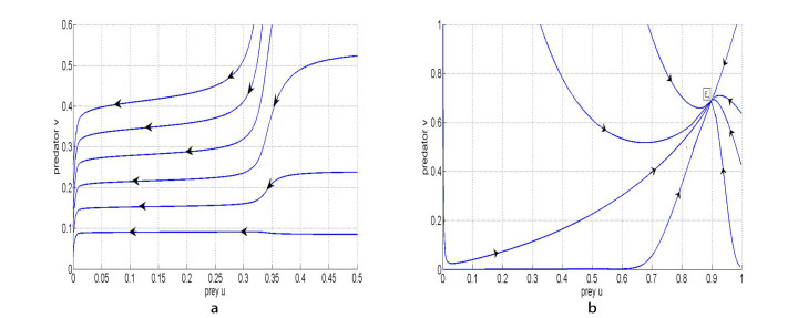
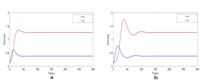
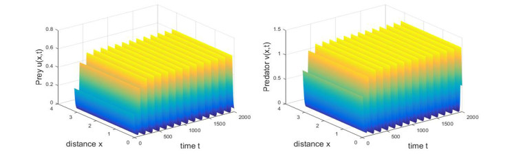
To portray the global stability of trivial steady state E0 and the positive constant steady state E∗, let a=1.35,b=0.01,c=1.353,d=0.5676,δ=1,h=0.28,ρ=0.045,s=0.001, by simple calculation, we are able to obtain (ρ+h−1)2<4(dh−ρ). It follows from Theorem 4.2 that E0 is globally asymptotically stable. It can be seen Figure 1a. Moreover, denote a=0.2,b=1.5,c=1.35,d=0.5676,δ=1,h=0.06,ρ=0.045,s=0.01, then the unique positive constant steady state E∗=(0.8984,0.6894) is globally asymptotically stable by Theorem 4.6. As shown in Figure 1b.
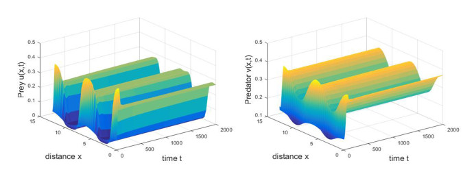
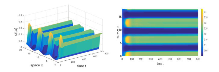
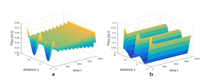
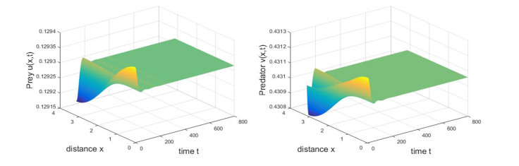
We consider the Turing instability with respect to the unique positive constant steady state E∗ of system (1.7) with τ=0. Let a=1.2,b=0.5,c=0.4,d=1.8,δ=0.15,h=0.161,ρ=0.5,s=0.2,d1=0.005,d2=0.5 and l=4. By simple calculation, we obtain that system (1.7) has a unique positive steady state E∗=(0.0527,0.1547). It follows from Theorem 4.4 that assumption (H1)∼(H3) and (H5)∼(H6) are satisfied, that is, the positive steady state E∗ for the ODE system is stable. However, for the PDE system, the positive steady state E∗ becomes unstable, and system (1.7) has a stable nonconstant steady state solution, which means that a Turing instability occurs. This is shown in Figure 2. It portrays that the population is irregularly distributed in space. We also observe that the system (1.7) has a stationary spatial pattern, that is shown in Figure 3. Moreover, choose d1=0.01, we are able to observe that under the effect of diffusion coefficients of d2, system (1.7) portrays different spatial patterns that can be periodic, stationary, as shown in Figure 4.
Firstly, we consider that the unique positive constant steady state E∗ of system (1.7) is locally asymptotically stable for all τ≥0. Let a=1,b=0.5,c=0.4,d=2,δ=0.15,h=0.01,ρ=0.5,s=0.2,d1=0.01,d2=0.02. By calculation, the positive constant steady state E∗=(0.3783,1.2611), the conditions (H1)∼(H4) and (H7) are satisfied. It follows from Theorem 4.5 that the unique positive constant steady state E∗ of system (1.7) is locally asymptotically stable for all τ≥0 in Figure 5.
Consider system (1.7) with the parameters a=1,b=0.5,c=0.4,d=2,δ=0.15,h=0.1,ρ=0.5,s=0.2,d1=0.01,d2=0.02 and l=1. Calculation shows that system (1.7) has a unique positive constant steady state E∗=(0.1293,0.4311). Hypothesis (H1)∼(H4) and (H8) satisfy for n=0, by calculation we have ω0=0.0652. It follows from Theorem 4.7 that homogeneous Hopf bifurcations occur at τj0≈6.1868+96.3679j for j∈N0. We use the forward Euler method to find numerical solutions to system (1.7) with τ=0,5.85,6.20, respectively. From Theorem 4.3, the unique positive constant steady state E∗=(0.1293,0.4311) of system (1.7) with τ=0 is locally asymptotically stable, it can be seen from Figure 6.
As shown in Figure 7 and 8, we observe sustained oscillations when delay τ crosses the critical value τ00≈6.1868. We have λ′(τ00)≈0.0035−0.0014i by Lemma 4.4. From Theorem 4.7, we know that if τ∈[0,τ00), then the equilibrium E∗=(0.1293,0.4311) is locally asymptotically stable. This is shown in Figure 7. And we conclude that the equilibrium E∗=(0.1293,0.4311) loses its stability and Hopf bifurcation occurs when τ crosses the critical value τ00. By calculation and Eq (5.16), we get C1(0)=−0.5076−1.4071i,μ2≈145.0286>0,β2≈−1.0152<0,T2≈3.9916>0.
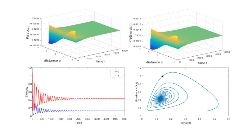
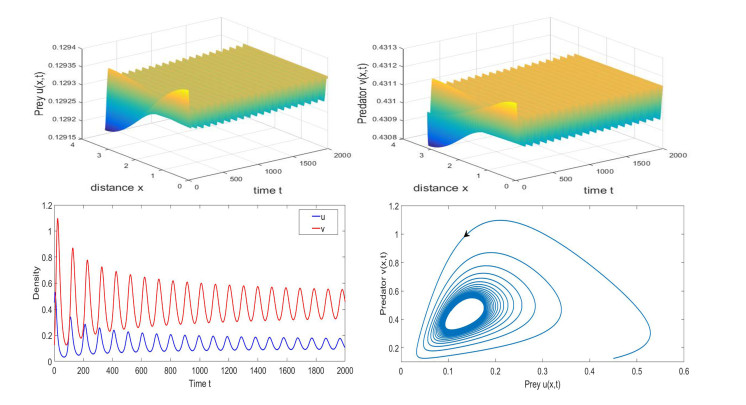
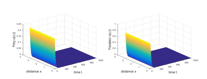
Hence, it follows from Theorem 5.1 that the direction of the bifurcation is forward, and the bifurcating period solutions are locally asymptotically stable. Moreover, the period of bifurcating periodic solutions increases. This is shown in Figure 8. If τ is increasing crosses the critical value τ01≈10.0462, a spatially inhomogeneous periodic solution occurs near the positive equilibrium E∗=(0.1293,0.4311). However, the bifurcating periodic solution bifurcating from the critical value τ01 must be unstable on the whole phase space since the characteristic equation always has roots with positive real parts for τ>τ00≈6.1868. This is shown in Figure 9. Besides, as τ increases further, with the same initial values, the solution of system (1.7) converges to (0,0), which implies that the increasing delay may cause the prey and predator to go extinct. As shown in Figure 10.
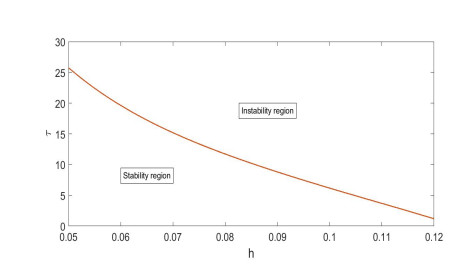
Considering the effect of nonlinear harvesting, we denote the parameters be the same as section 6.3 and h vary in [0.05,0.12]. The stability and instability regions of the unique positive constant steady state E∗ for system (1.7) is depicted by mapping the nonlinear harvesting to the critical value of the delay τ in Figure 11. We observe that the nonlinear harvesting effect parameter h increases from 0.05 and 0.12, the Hopf bifurcation is occurred for lower critical values of τ. Meanwhile, we observe that the harvesting effect parameter h has a significant effect on the stability of ecosystem.
In this paper, we focused on a delayed diffusive predator-prey system with food-limited and nonlinear harvesting effect. Firstly, in order to prove the global stability of the solution, we gave the existence of solution and priori bound. Meanwhile, we also derived the conditions of stability of the nonnegative constant steady state solution. Moreover, the global stability of the trivial and positive constant steady state is investigated. The conditions of Turing instability and Hopf bifurcation are obtained for system (1.7), respecitvely. For the positive constant steady state solution, it is demonstrated that Hopf bifurcation can be occurred when bifurcation parameter τ increases beyond a critical value. We derived the detailed formulas to determine the properties of Hopf bifurcation.
For the system (1.7), it follows from Theorem 4.2 and Theorem 4.6 that the trivial steady state E0 and the positive constant steady state E∗ are globally asymptotically stable under the certain conditions (Figure 1), respectively. From an ecological point of view, due to the food-limited in the natural environment, intraspecific competition in prey population increases, so nonlinear prey harvesting is taken into consideration. Increasing the harvesting effect parameter h properly can decrease the density of prey population so that relieve the pressure of intraspecific competition and the system becomes stable under the certain conditions. However, if h crosses a certain value, the density of prey population begins decreasing and may even become extinct (Figures 10 and 11). The diffusion induces the occurrence of Turing instability for the positive steady state E∗, which means that system (1.7) has a stable nonconstant steady state solution (Figures 2 and 3). Our results also reveal the fact that delay can induce very complex dynamics phenomenon, and a positive constant steady state E∗ is depicted to be locally asymptotically stable when the parameter τ is less than the critical value τ∗ (Figure 7), and a stable periodic solutions will bifurcate from the constant steady state E∗ (Figure 8), when the delay τ increase and it crosses through the critical value τ∗, which means that a stable and spatially homogeneous periodic solutions will occur at the critical value of delay τ∗, when the delay τ continues to increase to a certain value, spatially inhomogeneous periodic solution bifurcates from the positive constant steady state E∗ for system (1.7) (Figure 9). When the delay τ is larger, the solution of system (1.7) tends to (0,0), that is, the population becomes extinct eventually (Figure 10).
From the biological point of view, it is clear that delay, nonlinear harvesting and diffusion effect have a significant impact on the stability for ecosystem.
However, there exists many problems will need to be investigated for system (1.7). Firstly, the selection results of Turing patterns are obtained by weakly nonlinear analysis[29,30]. Secondly, the diffusion of the population is random and homogeneous in this paper, actually, individuals often perform a nonlocal diffusion or heterogeneous diffusion in the real world. Finally, spatial memory and cognition of animals has drawn much attention in the mathematical modeling of animal movement (i.e., memory-based diffusion)[42]. These problems will be investigated in the future.
We would like to express our gratitude to the referees for their valuable comments and suggestions that led to a truly significant improvement of the manuscript. The work is supported by the National Natural Science Foundation of China (11871475) and the Fundamental Research Funds for the Central University of Central South University (2019zzts212).
The authors declare that they have no conflict of interest.
| [1] | Chaperon I (1986) Theoretical Study of Coning Toward Horizontal and Vertical Wells in Anisotropic Formations: Subcritical and Critical Rates. SPE Annu Tech Conf Exhib, 5-8. |
| [2] |
Chierici GL, Ciucci GM, Pizzi G (1964) A Systematic Study of Gas and Water Coning By Potentiometric Models. J Pet Technol 16: 923-929. doi: 10.2118/871-PA

|
| [3] | Wheatley MJ (1985) An Approximate Theory of Oil/Water Coning. SPE Annual Technical Conference and Exhibition, Las Vegas, Nevada, USA, 22-26. |
| [4] | Al-Sikaiti SH, Regtien J (2008) Challenging Conventional Wisdom, Waterflooding Experience on Heavy Oil Fields in Southern Oman. World Heavy Oil Congr: 10-12. |
| [5] |
Karami M, Khaksar Manshad A, Ashoori S (2014) The Prediction of Water Breakthrough Time and Critical Rate with a New Equation for an Iranian Oil Field. Pet Sci Technol 32: 211-216. doi: 10.1080/10916466.2011.586960
|
| [6] |
Jiang X (2011) A review of physical modelling and numerical simulation of long-term geological storage of CO2. Appl Energy 88: 3557-3566. doi: 10.1016/j.apenergy.2011.05.004
|
| [7] |
Jung JY, Huh C, Kang SG, et al. (2013) CO2 transport strategy and its cost estimation for the offshore CCS in Korea. Appl Energy 111: 1054-1060. doi: 10.1016/j.apenergy.2013.06.055
|
| [8] | Buscheck TA, White JA, Chen M, et al. (2014) Pre-injection brine production for managing pressure in compartmentalized CO2 storage reservoirs. Energy Procedia 63, 5333-5340. |
| [9] |
González-Nicolás A, Cihan A, Petrusak R, et al. (2019) Pressure management via brine extraction in geological CO2 storage: Adaptive optimization strategies under poorly characterized reservoir conditions. Int J Greenhouse Gas Control 83: 176-185. doi: 10.1016/j.ijggc.2019.02.009
|
| [10] | Pongtepupathum W, Williams J, Krevor S, et al. (2017) Optimising Brine Production for Pressure Management During CO2 sequestration in the Bunter Sandstone of the UK Southern North Sea. Soc Pet Eng. |
| [11] | Tarrahi M, Afra S (2015) Optimization of Geological Carbon Sequestration in Heterogeneous Saline Aquifers through Managed Injection for Uniform CO2 Distribution. Carbon Management Technology Conference. |
| [12] |
Liao C, Liao X, Mu L, et al. (2017) Improving water-alternating-CO2 flooding of heterogeneous, low permeability oil reservoirs using ensemble optimisation algorithm. Int J Global Warming 12: 242-260. doi: 10.1504/IJGW.2017.084509
|
| [13] | Shamshiri H, Jafarpour B (2010) Optimization of Geologic CO2 Storage in Heterogeneous Aquifers Through Improved Sweep Efficiency. SPE International Conference on CO2 Capture, Storage, and Utilization held in New Orleans, Louisiana, 10-12. |
| [14] | Kazakis N, Pavlou A, Vargemezis G, et al. (2016) Seawater intrusion mapping using electrical resistivity tomography and hydrochemical data. An application in the coastal area of eastern Thermaikos Gulf, Greece. Sci Total Environ 543: 373-387. |
| [15] | Goldman M, Kafri U (2006) Hydrogeophysical applications in coastal aquifers. In: Vereecken H, Author, Applied Hydrogeophysics, Eds., Springer: Dordrecht, The Netherlands, 233-254. |
| [16] | Kuras O, Pritchard J, Meldrum P, et al. (2009) Monitoring hydraulic processes with automated time-lapse electrical resistivity tomography (ALERT): Compt Rendus Geosci 341: 868-885. |
| [17] | Dell'Aversana P, Rizzo E, Servodio R (2017) 4D borehole electric tomography for hydrocarbon reservoir monitoring. EAGE Conference and Exhibition, 2017: 1-5. |
| [18] | McNeice GW, Colombo D (2018) 3D inversion of surface to borehole CSEM for waterflood monitoring. SEG Int Expo Ann Meet, 878-880. |
| [19] | Bergmann P, Schmidt-Hattenberger C, Kiessling D, et al. (2012) Surface-downhole electrical resistivity tomography applied to monitoring of CO2 storage at Ketzin, Germany. Geophysics 77: B253-B267. |
| [20] |
Bergmann P, Schmidt-Hattenberger C, Labitzke1 T, et al. (2017) Fluid injection monitoring using electrical resistivity tomography—five years of CO2 injection at Ketzin, Germany. Geophys Prospect 65: 859-875. doi: 10.1111/1365-2478.12426
|
| [21] |
Schmidt-Hattenberger C, Bergmann P, Bö sing D, et al. (2013) Electrical resistivity tomography (ERT) for monitoring of CO2 migration-from tool development to reservoir surveillance at the Ketzinpilot site. Energy Procedia 37: 4268-4275. doi: 10.1016/j.egypro.2013.06.329
|
| [22] |
Descloitres M, Ribolzi O, Le Troquer Y (2003) Study of infiltration in a Sahelian gully erosion area using time-lapse resistivity mapping. Catena 53: 229-253. doi: 10.1016/S0341-8162(03)00038-9
|
| [23] | Dell'Aversana P, Servodio R, Bottazzi F, et al. (2019_a) Asset Value Maximization through a Novel Well Completion System for 3d Time Lapse Electromagnetic Tomography Supported by Machine Learning. Abu Dhabi Int Pet Exhib Conf. |
| [24] | Dell'Aversana P, Servodio R, Bottazzi F, et al, (2019_b). Asset Value Maximization through a Novel Well Completion System for 3d Time Lapse Electromagnetic Tomography Supported by Machine Learning. Soc Pet Eng J. |
| [25] | Bottazzi F, Dell'Aversana P, Molaschi C, et al. (2020) A New Downhole System for Real Time Reservoir Fluid Distribution Mapping: E-REMM, the Eni-Reservoir Electro-Magnetic Mapping System. Int Pet Technol Conf. |
| [26] | Brown RG (1956) Exponential Smoothing for Predicting Demand. Cambridge, Massachusetts: Arthur D. Little Inc 15. |
| [27] |
Saad EW, Prokhorov DV, Wunsch DC (1998) Comparative study of stock trend prediction using time delay, recurrent and probabilistic neural networks. IEEE T Neural Network 9: 1456-1470. doi: 10.1109/72.728395
|
| [28] |
Tealab A (2018) Time series forecasting using artificial neural networks methodologies: A systematic review. Future Comput Inform J 3: 334-340. doi: 10.1016/j.fcij.2018.10.003
|
| [29] |
Sherstinsky A (2020) Fundamentals of Recurrent Neural Network (RNN) and Long Short-Term Memory (LSTM) Network. Phys D 404: 132306. doi: 10.1016/j.physd.2019.132306
|
| [30] |
Kaelbling LP, Littman ML, Moore AW (1996) Reinforcement Learning: A Survey. J Artif Intell Res 4: 237-285. doi: 10.1613/jair.301
|
| [31] | Raschka S, Mirjalili V (2017) Python Machine Learning: Machine Learning and Deep Learning with Python, scikit-learn, and TensorFlow, 2nd Ed., PACKT Books. |
| [32] | Russell S, Norvig P (2016) Artificial Intelligence: A Modern approach, Global Edition, Pearson Education, Inc., publishing as Prentice Hall. |
| [33] | Machine learning workflows. Multidisciplinary applications using Python, 2021. Available from: https://www.researchgate.net/publication/348741974_Q_Learning_generic. |
| [34] |
Benson SM, Surles T (2006) Carbon dioxide capture and storage: an overview with emphasis on capture and storage in deep geological formations. Proc IEEE 94: 1795-1805. doi: 10.1109/JPROC.2006.883718
|
| [35] |
Christensen NB, Sherlock D, Dodds K (2006) Monitoring CO2 injection with cross-hole electrical resistivity tomography. Explor Geophys 37: 44-49. doi: 10.1071/EG06044
|
| [36] |
LaBrecque DJ, Miletto M, Daily W, et al. (1996) The effects of noise on Occam's inversion of resistivity tomography data. Geophysics 61: 538-548. doi: 10.1190/1.1443980
|
| [37] | Dell'Aversana P, Carbonara S, Vitale S, et al (2011) Quantitative estimation of oil saturation from marine CSEM data: A case history. First Break 29. |
| [38] | Befus KM (2017) Pyres: A Python Wrapper for Electrical Resistivity Modeling with R2. J Geophys Eng 15. |
| [39] | Binley A, A Kemna (2005) Electrical Methods, In: Hydrogeophysics by Rubin and Hubbard Eds., Springer, 129-156. |
| [40] | Binley A (2015) Tools and Techniques: DC Electrical Methods, In: Treatise on Geophysics, 2nd Ed., Schubert: Elsevier, 233-259. |
| [41] | Binley A (2016) R2 version 3.1 Manual. Lancaster, UK. Available from: http://es.lancs.ac.uk/people/amb/Freeware/freeware.htm. |
| [42] | PUNQ-S3 reservoir model, Imperial College of London. Available from: https://www.imperial.ac.uk/earth-science/research/research-groups/perm/standard-models/. |
| [43] | Archie GE (1950) Introduction to petrophysics of reservoir rocks. AAPG Bulletin 34: 943-961. |
| [44] |
Claerbout JF, Muir F (1973) Robust modeling with erratic data. Geophysics 18: 826-844. doi: 10.1190/1.1440378
|
| [45] |
Sagheer A, Kotb M (2019) Time series forecasting of petroleum production using deep LSTM recurrent networks. Neurocomputing 323: 203-213. doi: 10.1016/j.neucom.2018.09.082
|


Figures(16) / Tables(2)

Paolo Dell'Aversana. Reservoir prescriptive management combining electric resistivity tomography and machine learning[J]. AIMS Geosciences, 2021, 7(2): 138-161. doi: 10.3934/geosci.2021009

 DownLoad:
