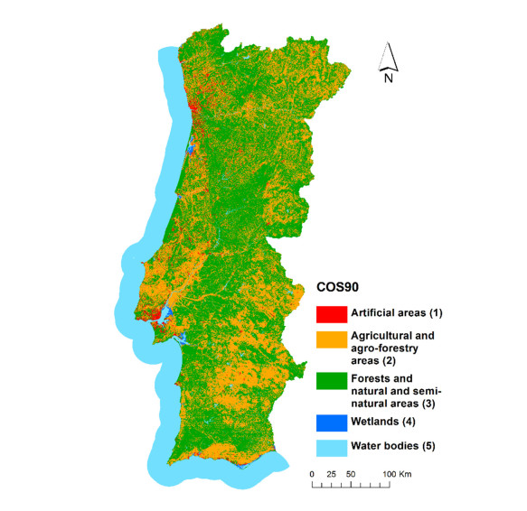
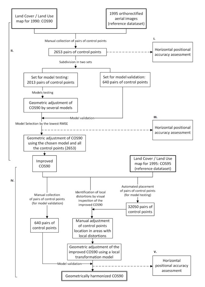
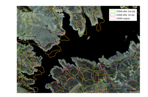
This paper describes an approach for harmonizing historical vector categorical maps with related modern maps. The approach aims at the correction of geometric distortions and semantic disagreements using alignment processes and analysis of thematic coherence. The harmonized version of the map produced by this approach can already be overlaid with other maps, what was unfeasible with the original map. The positional errors of the old map are reduced by two consecutive geometric adjustments, which use transformations usually available in most GIS software. The thematic consistency between the old and the modern map is achieved by harmonizing their classification systems and by the inclusion of specific contents missing in the early map, but represented in the modern map (e.g. small rivers). This approach was tested in the geometric and thematic harmonization of the Portuguese Land Cover/Land Use (LCLU) map for 1990 (COS90). In this test, the 1995 orthorectified aerial images and the 1995 LCLU map (COS95) were used as reference sources of higher positional accuracy, to align the COS90 map. COS90 was firstly adjusted with the 1995 aerial images by an NTV2 grid transformation, developed by the authors. Then, for reduction of the local distortions, the map resulting from the first transformation was aligned with the COS95 by a rubber-sheeting linear interpolation transformation. This geometric harmonization enabled a decrease of the Root Mean Square Error of COS90 from 204 meters to 13 meters. The thematic harmonization of COS90 enabled its comparison with modern related maps, and the integration of 201 river sections, that were missing because the specifications used in the production of the original map did not allow their representation.
Citation: Rita Nicolau, Nadiia Basos, Filipe Marcelino, Mário Caetano, José M. C. Pereira. Harmonization of categorical maps by alignment processes and thematic consistency analysis[J]. AIMS Geosciences, 2020, 6(4): 473-490. doi: 10.3934/geosci.2020026
This paper describes an approach for harmonizing historical vector categorical maps with related modern maps. The approach aims at the correction of geometric distortions and semantic disagreements using alignment processes and analysis of thematic coherence. The harmonized version of the map produced by this approach can already be overlaid with other maps, what was unfeasible with the original map. The positional errors of the old map are reduced by two consecutive geometric adjustments, which use transformations usually available in most GIS software. The thematic consistency between the old and the modern map is achieved by harmonizing their classification systems and by the inclusion of specific contents missing in the early map, but represented in the modern map (e.g. small rivers). This approach was tested in the geometric and thematic harmonization of the Portuguese Land Cover/Land Use (LCLU) map for 1990 (COS90). In this test, the 1995 orthorectified aerial images and the 1995 LCLU map (COS95) were used as reference sources of higher positional accuracy, to align the COS90 map. COS90 was firstly adjusted with the 1995 aerial images by an NTV2 grid transformation, developed by the authors. Then, for reduction of the local distortions, the map resulting from the first transformation was aligned with the COS95 by a rubber-sheeting linear interpolation transformation. This geometric harmonization enabled a decrease of the Root Mean Square Error of COS90 from 204 meters to 13 meters. The thematic harmonization of COS90 enabled its comparison with modern related maps, and the integration of 201 river sections, that were missing because the specifications used in the production of the original map did not allow their representation.

| [1] |
Mas JF (2005) Change Estimates by Map Comparison: A Method to Reduce Erroneous Changes Due to Positional Error. Trans GIS 9: 619-629. doi: 10.1111/j.1467-9671.2005.00238.x

|
| [2] | Luz A, Nunes A, Caetano M (2008) Proposta metodológica para a correcção das distorções geométricas da COS'90: resultados preliminares. In: Rocha JG, editor. Proceedings of the 10th ESIG—X Encontro de Utilizadores de Informação Geográfica. Oeiras Portugal, Universidade do Minho, 14. |
| [3] | Chrisman NR, Lester M (1991) A diagnostic test for error in categorical maps. In Proceedings of the Tenth International Symposium on Computer-Assisted Cartography—Auto-Carto 10. American Congress on Surveying and Mapping and American Society for Photogrammetry and Remote Sensing, Baltimore Maryland, 330-348. |
| [4] | Ware JM, Jones CB (1998) Matching and aligning features in overlayed coverages. In Laurini R, Makki K, Pissinou N, editors. Proceedings of 6th ACM International Symposium on Advances in Geographical Information Systems—ACM-GIS'98. Association for Computing Machinery, 28-33. |
| [5] |
Gaeuman D, Symanzik J, Schmidt JC (2005) A Map Overlay Error Model Based on Boundary Geometry. Geogr Anal 37: 350-369. doi: 10.1111/j.1538-4632.2005.00585.x
|
| [6] | Veregin HA (1989) Taxonomy of Error in Spatial Databases. Technical Report 89-12; Santa Barbara: U.S. National Center for Geographic Information and Analysis, University of California, 109. |
| [7] | Harvey F, Vauglin F (1996) Geometric match processing: Applying multiple tolerances. In Kraak MJ, Molenaar M, editors. Proceedings of the 7th International. Symposium on Spatial Data Handling: Advances in GIS Research II—SDH'96. Delft University of Technology, Delft, The Netherlands, 1: 13-29. |
| [8] | Galanda M, Koehnen R, Schroeder J, et al. (2005) Automated generalization of historical U.S. census units. In: Proceedings of the 8th ICA Workshop on Generalisation and Multiple Representation. International Cartographic Association, A Coruña, Spain, 10. |
| [9] |
Schorcht M, Krüger T, Meinel G (2016) Measuring Land Take: Usability of National Topographic Databases as Input for Land Use Change Analysis: A Case Study from Germany. ISPRS Int J Geo-Inf 5: 134. doi: 10.3390/ijgi5080134
|
| [10] |
Liu H, Zhao Z, Jezek KC (2004) Correction of Positional Errors and Geometric Distortions in Topographic Maps and DEMs Using a Rigorous SAR Simulation Technique. Photogramm Eng Remote Sens 70: 1031-1042. doi: 10.14358/PERS.70.9.1031
|
| [11] |
Schuurman N, Grund D, Hayes M, et al. (2006) Spatial/temporal mismatch: a conflation protocol for Canada Census spatial files. Can Geogr/Le Géogr Can 50: 74-84. doi: 10.1111/j.0008-3658.2006.00127.x
|
| [12] | Herrault P, Sheeren D, Fauvel M, et al. (2013) A comparative study of geometric transformation models for the historical "Map of France" registration. Geogr Tech 1: 34-46. |
| [13] | Schulze MJ, Thiemann F, Sester M (2014) Using Semantic Distance to Support Geometric Harmonisation of Cadastral and Topographical Data. ISPRS Ann Photogramm Remote Sens Spatial Inf Sci II-2, 15-22. |
| [14] | Brovelli MA, Minghini M (2012) Georeferencing old maps: a polynomial-based approach for Como historical cadastres. e-Perimetron 7: 97-110. |
| [15] | Barazzetti L, Brumana R, Oreni D, et al. (2014) Historical Map Registration via Independent Model Adjustment with Affine Transformations, In: Murgante B, Misra S, Rocha AMAC, et al. (Eds.), Computational Science and Its Applications—ICCSA 2014, Portugal: Springer, 44-56. |
| [16] | Boutoura C, Livieratos E (2006) Some fundamentals for the study of the geometry of early maps by comparative methods. e-Perimetron 1: 60-70. |
| [17] | Balletti C (2006) Georeference in the analysis of the geometric content of early maps. e-Perimetron 1: 32-42. |
| [18] | Bitelli G, Cremonini S, Gatta G (2009) Ancient map comparisons and georeferencing techniques: A case study from the Po River Delta (Italy). e-Perimetron 4: 221-233. |
| [19] | Dai Prà E, Mastronunzio M (2014) Rectify the river, rectify the map. Geometry and geovisualization of Adige river hydro-topographic historical maps. e-Perimetron 9: 113-128. |
| [20] | Caetano M, Pereira M, Carrão H, et al. (2008) Cartografia temática de ocupação/uso do solo do Instituto Geográfico Português. Mapp-Rev Int Cienc Tierra 126: 78-87. |
| [21] | Caetano M, Araújo A, Nunes V (2009) Proposta de conversão da nomenclatura da COS'90 para a da COS2007. Lisboa: Instituto Geográfico Português, 51. |
| [22] | Caetano M, Nunes A, Dinis J, et al. (2010) Carta de Uso e Ocupação do Solo de Portugal Continental para 2007 (COS2007v2.0): memória descritiva. Lisboa: Instituto Geográfico Português, 97. |
| [23] | DGT—Direção-Geral do Território (2018) Especificações técnicas da Carta de uso e ocupação do solo de Portugal Continental para 1995, 2007, 2010 e 2015. Lisboa: Direção-Geral do Território, 103. |
| [24] | FGDC—Federal Geographic Data Committee (1998) Geospatial Positioning Accuracy Standards. Part 3: National Standard for Spatial Data Accuracy. Available from: https://www.fgdc.gov/standards/projects/accuracy/part3/chapter3. |
| [25] | Guerra F (2000) 2W: new technologies for the georeferenced visualization of historic cartography. Int Arch Photogramm Remote Sens 33: 339-345. |
| [26] | Junkins D, Farley S (1995) NTv2 National Transformation Version 2—Developer's Guide. Canada: Geomatics Canada—Geodetic Survey Division, 27. |
| [27] |
White MS, Griffin P (1985) Piecewise linear rubber-sheet map transformations. Am Cartographer 12: 123-131. doi: 10.1559/152304085783915135
|
| [28] |
Saalfeld A (1985) A fast rubber-sheeting transformation using simplical coordinates. Am Cartographer 12: 169-173. doi: 10.1559/152304085783915072
|
| [29] | ESRI—Environmental Systems Research Institute (2016) ArcGIS for Desktop documentation About spatial adjustment rubbersheeting. Available from: https://desktop.arcgis.com/en/arcmap/10.3/manage-data/editing-existing-features/about-spatial-adjustment-rubbersheeting.htm. |
| [30] | Fuse T, Shimizu E, Morichi S (1998) A study on geometric correction of historical maps. Int Arch Photogramm Remote Sens 32: 543-548. |
| [31] | Balletti C (2000) Analytical and quantitative methods for the analysis of the geometrical content of historical cartography. Int Arch Photogramm Remote Sens 33: 30-37. |
| [32] | Shimizu E, Fuse T (2005) A Method for Visualizing the Landscapes of Old-Time Cities Using GIS. In: Okabe A (Eds.), GIS-based Studies in the Humanities and Social Sciences, CRC Press Taylor & Francis group, 265-277. |
Figures(3) / Tables(3)

Rita Nicolau, Nadiia Basos, Filipe Marcelino, Mário Caetano, José M. C. Pereira. Harmonization of categorical maps by alignment processes and thematic consistency analysis[J]. AIMS Geosciences, 2020, 6(4): 473-490. doi: 10.3934/geosci.2020026


 DownLoad: