Nexus between water, energy, food and climate change as challenges facing the modern global, European and Polish economy

Piotr F. Borowski; Piotr F. Borowski

doi:10.3934/geosci.2020022

AIMS Geosciences

2020, Volume 6, Issue 4: 397-421. doi: 10.3934/geosci.2020022

Previous Article Next Article

Review Special Issues

Nexus between water, energy, food and climate change as challenges facing the modern global, European and Polish economy

Piotr F. Borowski ^,

Warsaw University of Life Sciences. Institute of Mechanical Engineering, 166 Nowoursynowska str, 02-787 Warsaw, Poland

Received: 13 July 2020 Accepted: 23 September 2020 Published: 30 September 2020

The relationship between food, energy and water is an increasingly significant cross-sectoral and interdisciplinary relationship and has an impact on the management of enterprises operating in these sectors. Phenomena occurring in one sector are closely related to others and affect them. In the 21st century, each sector cannot be considered separately, as development and innovation necessitate a holistic view. New varieties of plants or animals are not only the domain of agriculture, but bioengineering and natural sciences. Plant cultivation or animal husbandry also requires knowledge of physics, chemistry, meteorological conditions and earth sciences, and human economic activity has an impact on the environment and progressive climate change. The article reviews and discusses the existing relationships and presents examples of solutions for reducing energy expenditure, reducing water consumption used in industry and agriculture.
- energy,
- water,
- food,
- nexus,
- chain,
- sustainability
Citation: Piotr F. Borowski. Nexus between water, energy, food and climate change as challenges facing the modern global, European and Polish economy[J]. AIMS Geosciences, 2020, 6(4): 397-421. doi: 10.3934/geosci.2020022

Related Papers:

Abstract

The relationship between food, energy and water is an increasingly significant cross-sectoral and interdisciplinary relationship and has an impact on the management of enterprises operating in these sectors. Phenomena occurring in one sector are closely related to others and affect them. In the 21st century, each sector cannot be considered separately, as development and innovation necessitate a holistic view. New varieties of plants or animals are not only the domain of agriculture, but bioengineering and natural sciences. Plant cultivation or animal husbandry also requires knowledge of physics, chemistry, meteorological conditions and earth sciences, and human economic activity has an impact on the environment and progressive climate change. The article reviews and discusses the existing relationships and presents examples of solutions for reducing energy expenditure, reducing water consumption used in industry and agriculture.

References

[1]	Mortada S, Abou Najm M, Yassine A, et al. (2018) Towards sustainable water-food nexus: an optimization approach. J Cleaner Prod 178: 408-418. doi: 10.1016/j.jclepro.2018.01.020
[2]	Tashtoush FM, Al-Zubari WK, Shah A (2019) A review of the water-energy-food nexus measurement and management approach. Int J Energ Water Res 3: 361-374. doi: 10.1007/s42108-019-00042-8
[3]	Schmidt JJ, Matthews N (2018) From state to system: Financialization and the water energy-food-climate nexus. Geoforum 91: 151-159. doi: 10.1016/j.geoforum.2018.03.001
[4]	Chang Y, Li G, Yao Y, et al. (2016) Quantifying the water-energy-food nexus: Current status and trends. Energies 9: 65. doi: 10.3390/en9020065
[5]	Dombrowsky I (2011) Water-Energy-Food: do we need a nexus perspective? The Baonn Nexus Conference, German Development Institute/Deutsches Institut für Entwicklungspolitik.
[6]	Kling CL, Arritt RW, Calhoun G, et al. (2017) Integrated assessment models of the food, energy, and water nexus: A review and an outline of research needs. Ann Rev Resour Econ 9: 143-163. doi: 10.1146/annurev-resource-100516-033533
[7]	Avraamidou S, Beykal B, Pistikopoulos IPE, et al. (2018) A hierarchical food-energy-water nexus (FEW-N) decision-making approach for land use optimization. Comput Aided Chem Eng 44: 1885-1890. doi: 10.1016/B978-0-444-64241-7.50309-8
[8]	Karnib A, Alameh A (2020) Technology-oriented approach to quantitative assessment of water-energy-food nexus. Int J Energ Water Res 4: 189-197. doi: 10.1007/s42108-020-00061-w
[9]	Wolfe ML, Ting KC, Scott N, et al. (2016) Engineering solutions for food-energy-water systems: it is more than engineering. J Environ Stud Sci 6: 172-182. doi: 10.1007/s13412-016-0363-z
[10]	Albrecht TR, Crootof A, Scott CA (2018) The Water-Energy-Food Nexus: A systematic review of methods for nexus assessment. Environ Res Lett 13: 043002. doi: 10.1088/1748-9326/aaa9c6
[11]	Nhamo L, Mabhaudhi T, Mpandeli S, et al. (2020) An integrative analytical model for the water-energy-food nexus: South Africa case study. Environ Sci Policy 109: 15-24. doi: 10.1016/j.envsci.2020.04.010
[12]	Endo A, Yamada M, Miyashita Y, et al. (2020) Dynamics of water-energy-food nexus methodology, methods, and tools. Curr Opin Environ Sci Health 13: 46-60. doi: 10.1016/j.coesh.2019.10.004
[13]	Nhamo L, Ndlela B, Nhemachena C, et al. (2018) The water-energy-food nexus: Climate risks and opportunities in southern Africa. Water 10: 567. doi: 10.3390/w10050567
[14]	Mpandeli S, Naidoo D, Mabhaudhi T, et al. (2018) Climate change adaptation through the water-energy-food nexus in southern Africa. Int J Environ Res Public Health 15: 2306. doi: 10.3390/ijerph15102306
[15]	Miralles-Wilhelm F (2016) Development and application of integrative modeling tools in support of food-energy-water nexus planning-a research agenda. J Environ Stud Sci 6: 3-10. doi: 10.1007/s13412-016-0361-1
[16]	Payet-Burin R, Kromann M, Pereira-Cardenal S, et al. (2019) WHAT-IF: an open-source decision support tool for water infrastructure investment planning within the water-energy-food-climate nexus. Hydrol Earth Syst Sci 23: 4129-4152. doi: 10.5194/hess-23-4129-2019
[17]	Borowski PF (2020) Adaptation strategies in energy sector enterprises. Available from: https://assets.researchsquare.com/files/rs-27944/v1/d2c58aec-2e48-4725-9866-6705e84c63b6.pdf.
[18]	Sarkodie SA, Owusu PA (2020) Bibliometric analysis of water-energy-food nexus: Sustainability assessment of renewable energy. Curr Opin Environ Sci Health 13: 29-34. doi: 10.1016/j.coesh.2019.10.008
[19]	United Nations (2020) World Economic Situation and Prospects, New York.
[20]	Nie Y, Avraamidou S, Xiao X, et al. (2019) A Food-Energy-Water Nexus approach for land use optimization. Sci Total Environ 659: 7-19. doi: 10.1016/j.scitotenv.2018.12.242
[21]	United Nations (2019) Population Division. World Population Prospects 2019. Department of Economic and Social Affairs.
[22]	Tidwell TL (2016) Nexus between food, energy, water, and forest ecosystems in the USA. J Environ Stud Sci 6: 214-224. doi: 10.1007/s13412-016-0367-8
[23]	Borowski PF (2017) Environmental pollution as a threats to the ecology and development in Guinea Conakry. Environ Prot Nat Resour 28: 27-32.
[24]	University of Leeds (2019) Amazon deforestation has a significant impact on the local climate in Brazil. Science Daily. Available from: https://www.sciencedaily.com/releases/2019/08/190830112813.htm.
[25]	M'mboroki KG, Wandiga S, Oriaso SO (2018) Climate change impacts detection in dry forested ecosystem as indicated by vegetation cover change in-Laikipia, of Kenya. Environ Monit Assess 190: 255. doi: 10.1007/s10661-018-6630-6
[26]	Baker JCA, Spracklen DV (2019) Climate Benefits of Intact Amazon Forests and the Biophysical Consequences of Disturbance. Front For Glob Change 2: 47. doi: 10.3389/ffgc.2019.00047
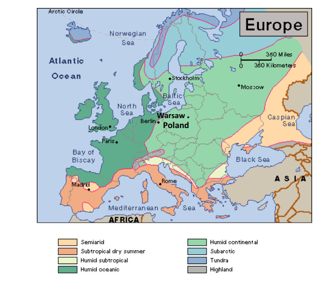
[27]	Robins R (2014) Lesson 2: Climate Regions of Europe. Available from: https://sites.google.com/site/6thgradeeuropeangeography/home/unit-5-the-geography-and-history-of-europe/lesson-2-climate-regions-of-europe.
[28]	Mann A, Reimann C, De Caritat P, et al. (2015) Mobile Metal Ion® analysis of European agricultural soils: bioavailability, weathering, geogenic patterns and anthropogenic anomalies. Geochem Explor Environ Anal 15: 99-112. doi: 10.1144/geochem2014-279
[29]	Poland Country Commercial Guide (2019) Poland-Environmental Technologies. Available from: https://www.export.gov/article?series=a0pt0000000PAuiAAG&type=Country_Commercial__kav.
[30]	Konikow LF, Kendy E (2005) Groundwater depletion: A global problem. Hydrogeol J 13: 317-320. doi: 10.1007/s10040-004-0411-8
[31]	Bartolino JR, Cunningham WL (2003) Ground-water depletion across the nation. US Geological Survey.
[32]	Kundzewicz ZW, Piniewski M, Mezghani A, et al. (2018) Assessment of climate change and associated impact on selected sectors in Poland. Acta Geophys 66: 1509-1523. doi: 10.1007/s11600-018-0220-4
[33]	Słyś D, Kordana S, Dziopak J (2015) The Law Regulations on the Subject of Rainwater Management in Poland. In: Hlavínek P, Zeleňková M (eds), Storm Water Management. Springer Hydrogeology. Springer, Cham.
[34]	Mioduszewski W (2014) Small (natural) water retention in rural areas. J Water Land Dev 20: 19-29. doi: 10.2478/jwld-2014-0005
[35]	Grey D, Sadoff CW (2007) Sink or swim? Water security for growth and development. Water Policy 9: 545-571. doi: 10.2166/wp.2007.021
[36]	SEJM (2017) Dz.U. 2017 poz. 1566-Prawo Wodne (Water Law). Available from: http://isap.sejm.gov.pl/isap.nsf/DocDetails.xsp?id=WDU20170001566.
[37]	Pierzgalski E (2018) New Water Act in Poland-Changes and Dilemmas. EU Agrar Law 7: 17-22. doi: 10.2478/eual-2018-0004
[38]	FAO-Food and Agriculture Organization of the United Nation (1980) The Law of International Resources, Rome.
[39]	Commission of the European Communities (2000) Directive 2000/60/EC of the European Parliament and of the Council of 23 October 2000 establishing a framework for Community action in the field of water policy. Available from: http://data.europa.eu/eli/dir/2000/60/2014-11-20.
[40]	Publications Office of the European Union (2019) Climate change in the agriculture sector in Europe, EEA Report.
[41]	Nawab A, Liu G, Meng F, et al. (2019) Urban energy-water nexus: spatial and inter-sectoral analysis in a multi-scale economy. Ecol Modell 403: 44-56. doi: 10.1016/j.ecolmodel.2019.04.020
[42]	United States Environmental Protection Agency (2017) Climate Impacts on Agriculture and Food Supply. Available from: www.epa.gov.
[43]	Patuk I, Hasegawa H, Borodin I, et al. (2020) Simulation for Design and Material Selection of a Deep Placement Fertilizer Applicator for Soybean Cultivation. Open Eng 10: 733-743.
[44]	Hendrickson JR, Hanson JD, Tanaka DL, et al. (2008) Principles of integrated agricultural systems: Introduction to processes and definition. Renew Agric Food Syst 23: 265-271. doi: 10.1017/S1742170507001718
[45]	Instytut Ochrony Środowiska (2020) Polityka klimatyczna z perspektywy Polski. Available from: https://ios.edu.pl/instytut-ochrony-srodowiska/polityka-klimatyczna-z-perspektywy-polski/.
[46]	Przybylak R, Oliński P, Koprowski M, et al. (2020) Droughts in the area of Poland in recent centuries in the light of multi-proxy data. Clim Past 16.
[47]	Działania w dziedzinie klimatu. Skutki zmian klimatu. Available from: https://ec.europa.eu/clima/change/consequences_pl.
[48]	Falling crop yields may lead to higher food prices and rise in hunger, Far Easter Agriculture. Available from: https://fareasternagriculture.com/crops/agriculture.
[49]	Bell A, Matthews N, Zhang W (2016) Opportunities for improved promotion of ecosystem services in agriculture under the Water-Energy-Food Nexus. J Environ Stud Sci 6: 183-191. doi: 10.1007/s13412-016-0366-9
[50]	Burkhead TR, Klink VP (2018) American agricultural commodities in a changing climate. AIMS Agric Food 3: 406-425. doi: 10.3934/agrfood.2018.4.406
[51]	Feola G, Lerner AM, Jain M, et al. (2015) Researching farmer behaviour in climate change adaptation and sustainable agriculture: Lessons learned from five case studies. J Rural Stud 39: 74-84. doi: 10.1016/j.jrurstud.2015.03.009
[52]	Gustafson RJ (1988) Fundamentals of electricity for agriculture, (Ed. 2), American Society of Agricultural Engineers, USA.
[53]	Bardi U, El Asmar T, Lavacchi A (2013) Turning electricity into food: the role of renewable energy in the future of agriculture. J Cleaner Prod 53: 224-231. doi: 10.1016/j.jclepro.2013.04.014
[54]	Bloch-Michalik M, Gaworski M (2015) A proposition of management of the waste from biogas plant cooperating with wastewater treatment. Agron Res 13: 455-463.
[55]	Gutiérrez AS, Eras JJC, Hens L, et al. (2020) The energy potential of agriculture, agroindustrial, livestock, and slaughterhouse biomass wastes through direct combustion and anaerobic digestion. The case of Colombia. J Cleaner Prod 2020: 122317
[56]	Publications Office of the European Union (2020) Towards an Inclusive Energy Transition in the European Union. Luxembourg.
[57]	Borowski PF (2020) Zonal and Nodal Models of energy market in European Union. Energies 13: 4182. doi: 10.3390/en13164182
[58]	Owusu PA, Sarkodie SA (2016) A review of renewable energy sources, sustainability issues and climate change mitigation. Cogent Eng 3: 1167990.
[59]	United Nations Development Programme (2019) Human Development Reports 2019. Available from: http://hdr.undp.org/sites/default/files/hdr2019.pdf.
[60]	The International Energy Efficiency Scorecard. Available from: https://www.aceee.org/portal/national-policy/international-scorecard.
[61]	Taghizadeh-Hesary F, Rasoulinezhad E, Yoshino N (2019) Energy and food security: Linkages through price volatility. Energy Policy 128: 796-806. doi: 10.1016/j.enpol.2018.12.043
[62]	Reid G (2020) The Six Energy Paradoxes that slow the sector's progress. Available from: https://energypost.eu/the-six-energy-paradoxes-that-slow-the-sectors-progress/.
[63]	Arrobbio O, Padovan D (2018) A vicious tenacity: The efficiency strategy confronted with the rebound effect. Front Energy Res 6: 114. doi: 10.3389/fenrg.2018.00114
[64]	Dharshing S, Hille SL (2017) The Energy Paradox Revisited: Analyzing the Role of Individual Differences and Framing Effects in Information Perception. J Consum Policy 40: 485-508. doi: 10.1007/s10603-017-9361-0
[65]	Herring H (2006) Confronting Jevons' paradox: does promoting energy efficiency save energy. Int Assoc Energy Econ Newsl 15: 14-15.
[66]	Borowski PF (2019) Adaptation strategy on regulated markets of power companies in Poland. Energy Environ 30: 3-26. doi: 10.1177/0958305X18787292
[67]	Igliński B (2019) Hydro energy in Poland: the history, current state, potential, SWOT analysis, environmental aspects. Int J Energ Water Res 3: 61-72. doi: 10.1007/s42108-019-00008-w
[68]	Ministerstwo Rolnictwa i Rozwoju Wsi (2019) Rolnictwo i gospodarka żywnościowa w Polsce. Available from: https://www.gov.pl/web/rolnictwo/rolnictwo-i-gospodarka-zywnosciowa-w-polsce.
[69]	Global Compact Network Poland (2018) Zasoby wodne w Polsce i możliwości rozwoju „małej" energetyki wodnej. Available from: https://ungc.org.pl/info/zasoby-wodne-polsce-mozliwosci-rozwoju-malej-energetyki-wodnej/.
[70]	Yah NF, Oumer AN, Idris MS (2017) Small scale hydro-power as a source of renewable energy in Malaysia: A review. Renewable Sustainable Energy Rev 72: 228-239. doi: 10.1016/j.rser.2017.01.068
[71]	Markkanen S, Braeckman JP, Souvannaseng P (2020) Mapping the evolving complexity of large hydropower project finance in low and lower-middle income countries. Green Financ 2: 151-172. doi: 10.3934/GF.2020009
[72]	Mazano-Agugliaro F, Taher M, Zapata-Sierra A, et al. (2017) An overview of research and energy evolution for small hydropower in Europe. Renewable Sustainable Energy Rev 72: 228-239. doi: 10.1016/j.rser.2017.01.068
[73]	Sołtuniak J (2016) Wpływ suszy hydrologicznej na inwestycje w energetyce wodnej. Możliwości zapobiegania skutkom suszy. Gospodarka Praktyce Teorii 44: 77-91.
[74]	Park H, Kim W (2019) Water industry: water-energy-health nexus. Environ Sci Pollut Res 26: 1013-1014. doi: 10.1007/s11356-018-3529-2
[75]	Lewandowska A, Piasecki A (2019) Selected aspects of water and sewage management in Poland in the context of sustainable urban development. Bull Geogr Socio-economic Ser 45: 149-157.
[76]	Endo A, Tsurita I, Burnett K, et al. (2017) A review of the current state of research on the water, energy, and food nexus. J Hydrol Reg Stud 11: 20-30. doi: 10.1016/j.ejrh.2015.11.010
[77]	Pracownia Zrównoważonego Rozwoju. Creating Interfaces. Available from: http://www.pzr.org.pl/portfolio/creating-interfaces/.
[78]	Eksperci przed światowym dniem wody (2020) Available from: https://naukawpolsce.pap.pl/aktualnosci/news%2C81311%2Ceksperci-przed-swiatowym-dniem-wody-chcesz-oszczedzac-wode-oszczedzaj.
[79]	Abdul NAK, Jayakumar R, Tamilmani G (2013) Recirculating aquaculture systems, Available from: http://www.eprints.cmfri.org.in/9712.
[80]	Borowski PF, Zalewski W (2014) Quality and innovation in recirculating aquaculture systems. Przem Spoż 68: 26-27.
[81]	Borowski PF, Zalewski W (2016) Innovation in Aquaculture to Ensure Healthy Fish Production. Inż Przetw Spoż 2: 15-18.
[82]	Landa-Cansigno O, Behzadian K, Davila-Cano DI, et al. (2020) Performance assessment of water reuse strategies using integrated framework of urban water metabolism and water-energy-pollution nexus. Environ Sci Pollut Res 27: 4582-4597. doi: 10.1007/s11356-019-05465-8
[83]	Bregnballe J (2015) A Guide to Recirculation Aquaculture. FAO and EUROFISH.
[84]	Ghisellini P, Protano G, Viglia S, et al. (2014) Integrated agricultural and dairy production within a circular economy framework. A comparison of Italian and Polish farming systems. J Environ Account Manag 2: 367-384.
[85]	Bożym M, Florczak I, Zdanowska P, et al. (2015) An analysis of metal concentrations in food wastes for biogas production. Renewable Energy 77: 467-472. doi: 10.1016/j.renene.2014.11.010
[86]	Wiśniewski K, Wardal WJ (2017) Wpływ stanu technicznego i nakładów finansowych na wybór sposobu modernizacji obory zgodnie ze standardami UE. Probl Inżynierii Rolniczej 25: 83-98.
[87]	Broucek J, Uhrincat M, Mihina S, et al. (2017) Dairy Cows Produce Less Milk and Modify Their Behaviour during the Transition between Tie-Stall to Free-Stall. Animals 7: 16. doi: 10.3390/ani7030016
[88]	Wisniewski K, Fornalczyk P (2012) Wpływ modernizacji budynków krów mlecznych na ich funkcjonalność na przykładzie obory krów mlecznych w fermie SGGW Obory-Goździe. Architectura 11: 69-76.
[89]	Anna Ferrari (2020) The milk war-The New Federalist. Available from: https://www.thenewfederalist.eu/the-milk-war?lang=fr.
[90]	Gaworski M, Leola A (2014) Effect of technical and biological potential on dairy production development. Agron Res 12: 215-222.

Reader Comments

Your name:*

Email:*
© 2020 the Author(s), licensee AIMS Press. This is an open access article distributed under the terms of the Creative Commons Attribution License (http://creativecommons.org/licenses/by/4.0)