
Citation: J. Brian Anderson, Jack Montgomery, Dan Jackson, Michael Kiernan, Chao Shi. Auburn University National Geotechnical Experimentation Site in Piedmont Residuum[J]. AIMS Geosciences, 2019, 5(3): 645-664. doi: 10.3934/geosci.2019.3.645
[1] | Jinhua Zhou, Shan Jia, Jinbao Chen, Meng Chen . Motion and trajectory planning modeling for mobile landing mechanism systems based on improved genetic algorithm. Mathematical Biosciences and Engineering, 2021, 18(1): 231-252. doi: 10.3934/mbe.2021012 |
[2] | Rongmei Geng, Renxin Ji, Shuanjin Zi . Research on task allocation of UAV cluster based on particle swarm quantization algorithm. Mathematical Biosciences and Engineering, 2023, 20(1): 18-33. doi: 10.3934/mbe.2023002 |
[3] | Smita Shandilya, Ivan Izonin, Shishir Kumar Shandilya, Krishna Kant Singh . Mathematical modelling of bio-inspired frog leap optimization algorithm for transmission expansion planning. Mathematical Biosciences and Engineering, 2022, 19(7): 7232-7247. doi: 10.3934/mbe.2022341 |
[4] | Jiguang Li, Mingyang Xie, Yanfei Dong, Hucheng Fan, Xin Chen, Gaomin Qu, Zhanfeng Wang, Peng Yan . RTPN method for cooperative interception of maneuvering target by gun-launched UAV. Mathematical Biosciences and Engineering, 2022, 19(5): 5190-5206. doi: 10.3934/mbe.2022243 |
[5] | Siyuan Shen, Xing Zhang, Wenjing Yan, Shuqian Xie, Bingjia Yu, Shizhi Wang . An improved UAV target detection algorithm based on ASFF-YOLOv5s. Mathematical Biosciences and Engineering, 2023, 20(6): 10773-10789. doi: 10.3934/mbe.2023478 |
[6] | Baoye Song, Shumin Tang, Yao Li . A new path planning strategy integrating improved ACO and DWA algorithms for mobile robots in dynamic environments. Mathematical Biosciences and Engineering, 2024, 21(2): 2189-2211. doi: 10.3934/mbe.2024096 |
[7] | Zhen Yang, Junli Li, Liwei Yang, Qian Wang, Ping Li, Guofeng Xia . Path planning and collision avoidance methods for distributed multi-robot systems in complex dynamic environments. Mathematical Biosciences and Engineering, 2023, 20(1): 145-178. doi: 10.3934/mbe.2023008 |
[8] | Eric Ruggieri, Sebastian J. Schreiber . The Dynamics of the Schoener-Polis-Holt model of Intra-Guild Predation. Mathematical Biosciences and Engineering, 2005, 2(2): 279-288. doi: 10.3934/mbe.2005.2.279 |
[9] | Li-zhen Du, Shanfu Ke, Zhen Wang, Jing Tao, Lianqing Yu, Hongjun Li . Research on multi-load AGV path planning of weaving workshop based on time priority. Mathematical Biosciences and Engineering, 2019, 16(4): 2277-2292. doi: 10.3934/mbe.2019113 |
[10] | Zhen Zhou, Chenchen Geng, Buhu Qi, Aiwen Meng, Jinzhuang Xiao . Research and experiment on global path planning for indoor AGV via improved ACO and fuzzy DWA. Mathematical Biosciences and Engineering, 2023, 20(11): 19152-19173. doi: 10.3934/mbe.2023846 |
In this paper, we consider the planning of an unmanned aerial vehicle (UAV) fleet mission problem with highly dynamic and unpredictable environment constraints [1,2,3,4,5]. Typical disruptions in urban deliveries by UAVs (characterized by frequent stop-and-go movements, low consolidation, and frequent re-scheduling), may be caused by changes in the order by customers, or shifting weather conditions (e.g., a sharp drop in temperature, icing of propellers, turbulence), which affect the energy consumption of UAVs and cause their shorter range due to the depletion of batteries [6,7]. For that reason, the routing of a UAV fleet in a partially known and unpredictable environment should guarantee a reactive on-line determined contingency reaction.
The UAVs' routes can be determined in the course of proactive planning [8] and generated in offline mode or in reactive planning [9,10], then executed in the online mode. Routes determined in proactive planning guarantee the achievement of the planned mission's goal for the environment's parameters, which change at predetermined intervals. Scenarios corresponding to planned reactive rules do not guarantee the existence of reactive end-to-end paths employed in the routing process while adapting it to changes in the environment during mission execution [2,6,10,11,12,13,14,15,16,17,18]. In particular, the reactive routing strategies linking the "route discovery (proactive route planning)" and "route maintenance (reactive rules adopting)" concepts [19] are responsible for UAV robustness to the changes that appear in the urban distribution context. In this context, our study focuses on reactive planning [20,21] of deliveries by a UAV fleet, which are resistant to sudden changes in weather conditions and unforeseen changes in the delivery schedules.
The originality of the paper results from its merging of the proactive and reactive planning of missions of UAV fleet. The developed models allow for predictive (i.e., taking into account forecasted weather conditions changing) and reactive (i.e., enabling interruption of a drone's mission) planning of delivery missions in terms of the constraint satisfaction problem [6,22,23] and the easy implementation of the proposed genetic algorithm in a commercially available constraint programming environment, e.g., IBM ILOG.
The paper is structured as follows. Section 2 presents the state of art. The approach to UAV mission contingency planning is presented in Section 3. The declarative model for reactive planning of deliveries by UAV fleets according to the constraint satisfaction problem is described in Section 4. Sufficient conditions guaranteeing the existence of a non-empty space of admissible solutions and, consequently, a reduction in the time expenditure incurred on the assessment of the weather changes are outlined in Section 5. The structure and operation of the developed genetic algorithm are presented in Section 6. The results of the conducted experiments regarding implementation of an accurate and approximate approach to UAV fleet mission planning are discussed in Section 7. Final conclusions are stated in Section 8, followed by suggestions for future research.
UAV mission planning issues play a key role in supply management systems in distributed networks belonging to the VRP class of NP-hard computational complexity [2,24]. Consequently, the sub-problems of routing and scheduling occurring in them also encounter a combinatorial explosion barrier, forcing the use of approximate solution methods. The goal is to identify a set of routes for a fleet of vehicles that optimizes some underlying objective function while subject to problem-specific constraints [25,26,27,28,29]. These efforts, according to the current taxonomy of available route planning methods, can be partitioned into two main categories: approximation and exact methods [6,26,30,31,32,33,34].
In general planning of the UAV path comes down to finding the path connecting the starting point with the destination that guarantees the fulfillment of the UAV operational requirements within the specified UAV flight constraints. Problems of this type undertaken in the area of UAV routing, i.e., VRP class problems [1,5], are formulated for various assumptions covering both the topography and the presence of obstacles. The topography, related to, e.g., mountainous and/or urbanized areas, influences the changes of the flight trajectory level, while the presence of stationary and/or dynamic obstacles makes it impossible to keep the straight shape of the trajectory [35]. Limitations of this type, force the inclusion of many new variables multiplying the complexity of UAVs trajectory planning problems, thus implying the need to use metaheuristic algorithms. The underlying nature-inspired algorithms such as the Bath algorithm, particle swarm optimization (PSO), artificial bee colony (ABC) algorithm, ant colony algorithm (ACO), grey wolf algorithm, etc. compete in terms of their convergence accuracy and proceeding efficiency [36,37,38].
Many works dealing with the problem of UAV routing, in particular those related to the use of UAVs in situations related to the monitoring of reservoirs, fields and forests, as well as flood victims support, assume UAV moves over flat terrain without obstacles that exclude the linear shape of their trajectory. In situations of this type, assuming that the UAV takes off vertically with the collected goods and also lands vertically in order to unload it, the problem of UAV routing boils down to determining the appropriate wind correction angle, correcting its drift [24]. Assuming these assumptions, this work addresses the problem of re-planning a UAV route in situations where sudden changes in wind direction and its intensity go beyond the fluctuation ranges adopted at the stage of proactive route planning.
An approximation method attempts to find the best possible solution while providing no guarantees as to the quality of that solution, i.e., it prefers quick solutions over optimal ones. In turn, an exact method is guaranteed to find the best solution to the problem given enough time, i.e., it is oriented toward the search for the optimal solution at the expense of the time incurred to obtain it. In the approximation approach, there are methods that implement heuristic algorithms (e.g., metaheuristics-driven ones, such as variable neighborhood search (VNS), simulated annealing (SA), and tabu search (TS)); population algorithms, such as PSO, ACO, ABC and evolutionary algorithms, such as memetic algorithms (MMA), and genetic algorithm (GA)) [26,30,32,34].
The exact approach leverages intelligent forms of enumerative search, such as dynamic programming (DP), mixed integer linear programming (MILP), branch-and-bound (BB), and constraint programming (CP) [6,31,33]. All of the above-mentioned approaches are supplemented by computer simulation tools, such as flight simulators [37,39,40].
There is a growing trend in research aimed at developing an interactive tool dedicated to online planning missions carried out by UAV teams, as reflected in numerous publications [12,13,16,22]. The aim of this research is to devise solutions that enable proactive and/or reactive planning of UAV missions in situations caused, for instance, by contingency planning in dynamic environments, i.e., decision support tools facilitating analysis and different scenarios comparison. Besides emergency situations, such tools can be helpful in various fields of application, e.g., reconnaissance and mapping, package delivery and delivery communication capabilities, healthcare and so on [3,4,12,13,18].
The UAV mission planning problems encountered in practice are characterized by a large variety of parameters, constraints, and specific evaluation criteria. Some examples of possible differences are listed in the following exemplary sets:
● parameters specifying UAVs (e.g., maximum loading capacity, maximum energy capacity, empty weight, payload weigh, ground speed, and aerodynamic drag coefficient), environmental conditions (e.g., weather forecasts including wind speed and direction, air density, temperature drizzle, or snowfall), and distribution network topology (e.g., number of delivery points, number of depots, and distances between delivery points and depots);
● constraints determining UAVs trajectories (e.g., to avoid collisions, a UAV is configured with at least one flight corridor and flight path), battery durability, delivery volumes, delivery periods, and changing weather conditions;
● evaluation criteria used to determine UAV fleet routings that guarantee the maximum benefits with the shortest total path, in particular, the maximum travel distance (limited by the capacity of the battery used), the minimum length of the sum of the flight path of each UAV, timely deliveries, resistance to changes in weather conditions, and/or service delivery deadlines.
As already mentioned, problems of this type belong to the category of NP-hard problems. This means that instances of such problems encountered in practice (due to their size as well as the number and variety of characteristics describing them) can be resolved within a reasonable time interval using approximate methods. In that context, the exact (i.e., optimal) solutions achieved in a similar time frame by exact methods refer, however, only to the small size instances out of practical significance. It is also easy to see that, in general, it is difficult to say which approach is best used for a given problem instance. The literature is rather scarce on this topic. Therefore, the research gap in this field is the motivation behind our research aimed at the implementation of selected methods representing both the approximate and exact approaches to compare them on using an arbitrarily selected example of a UAV fleet planning problem.
The comparison included CP as representative of the exact approach and GA as representative of the approximate approach. CP is a paradigm for solving combinatorial problems according to which users declaratively state the constraints on the feasible solutions for a set of decision variables. The acceptable solution sought is the set of decision variables values satisfying all the constraints [6,22,27]. It is worth emphasizing that CP is more general than MILP, allowing variable types beyond integer and continuous (e.g., interval and set variables), and dropping the restriction of linearity in the constraints and objective function. In turn, the GA, being the representative of evolutionary algorithms, is a search technique inspired by evolutionary biology such as inheritance, mutation, selection, and crossover used in computing to find true or approximate solutions to optimization and search problems [41,42,43]. Carrying out appropriate computer experiments allows to judge which approach is faster for which size of the selected instance of the UAV mission planning problem.
We consider a distribution network, which is modeled by the graph G=(N,E) where N={N1,…,Nλ,…,Nn} signifies the set of n=|N| nodes (distinguishing N1 node representing a base and {N2,…,Nn} nodes representing delivery points), and E={(Ni,Nj)|i,j∈{1,…,n},i≠j} signifies the set of edges determining the possible connections between nodes. Given a fleet of UAVs U={U1,…,Uk,…,UK} that delivers to the points {N2,…,Nn}, to each delivery point Nλ an ordered quantity of goods zλ∈N (taken from the base N1) should be transported. Deliveries are made as part of the mission S, which consists of sub-missions lS (i.e., delivery plans that include a single course of UAVs: base-delivery points-base). Z denotes a sequence consisting of variables zλ : Z =(z1,…,zn). It is assumed that all required goods should be delivered in the given horizon time H. The amount of goods delivered during one sub-mission lS by the Uk to the delivery point Nλ is determined by the variable lckλ∈N. lC is a sequence : lC=(lc11,…,lcK1,…,lc1n,…,lcKn) determining the payload weight delivered by fleet U. Variable Qk denotes the payload capacity of Uk (amount of goods transported by Uk cannot exceed Qk). Moreover, each Uk is described by the following technical parameters: battery capacity CAP, airspeed va, drag coefficient CD, front surface A, and UAV width b. Time spent on take-off and landing Uk on delivery point Nλ is indicated by variable wλ∈N. Note that lU⊆U denotes a set of UAVs used during sub-mission lS. The moment when the Uk∈lU arrives to the delivery point Nλ during sub-mission lS is indicated by variable lykλ∈N [s]. In that context, the sequence lY consisting of moments lykλ, is called the schedule of the fleet lU : lY=(ly11,…,lyK1,…,ly1n,…,lyKn).
We assume that the variable tβ,λ∈N determines traveling time between nodes Nβ, Nλ, where: (Nβ,Nλ)∈E, and routes of Uk∈lU during sub-mission lS are represented by sequences: lπk=(Nk1,…,Nki,Nki+1,…,Nkμ), where: ki∈{1,..,n}, (Nki,Nki+1)∈E. lΠ denotes a sequence of UAVs routes executed during sub-mission lS : lΠ=(lπ1,…,lπk,…,lπK) (in cases when Uk∉lU then lπk=△). The delivery plan of one UAV sub-mission lS is defined as a sequence: lS=(lU,lΠ,lY,lC).
It is assumed that a plan of a UAV sub-mission lS is implemented under specific weather conditions, i.e., the weather forecast is known for each sub-mission lS. The forecasted weather conditions are described by the set F of pairs composed of direction θ and wind speed vw (θ,vw)∈F, i.e., F is defined as follows: F={(θ,vw)|θ∈[0°,360°),vw∈[0,F(θ)]}. Where F(θ) is a function that's values determine the maximum forecasted wind speed for given direction θ. The weather conditions determine the admissibility of the adopted sub-mission's plan lS, i.e., they determine whether during its implementation, the batteries of UAVs will not be prematurely discharged.
A function Yk,l(θ) determines the borderline wind speed (for a given direction θ), which guarantees the successful completion of the delivery plan by the Uk during sub-mission lS in the distribution network G : Yk,l(θ)=maxΓk,l(θ), where: Γk,l(θ) – set of wind speed's values vw for a given direction θ, for which the batteries of Uk is not discharged. The sub-mission's plan lS is assumed [14] to be resistant to the forecast weather conditions F if the boundary wind Yk,l(θ) of all Uk∈lU in any direction θ does not exceed the forecasted value Z(θ) : ∀Uk∈lU∀θ∈[0°,360°)Yk,l(θ)≥F(θ).
The implementation of the designated mission S may be subject to various disturbances IS. Among them, there are sudden changes in the weather (beyond the expected F∗(θ) range), and changes in orders Z), order changes (increase /decrease amount of ordered deliveries Z∗), changes in the number of delivery points served (changing the structure of the network G∗). The UAV fleet, when performing the mission plan S, meets a disturbance IS(t∗)- covering one of the cases: the weather F∗(θ), the network G∗, orders Z∗, at the time t∗. In such situations, it becomes necessary to answer the question: Does a re-route plan exist for mission S∗ that guarantees timely deliveries in a given time horizon H and at acceptable battery level? To illustrate the motivation behind our approach, let us consider a distribution network from Figure 1a) covering an area of 100 km2 and containing 39 delivery points (nodes N2,…,N40).
The goods are delivered by a fleet of UAVs, which is stationed in the base N1 –technical parameters of UAVs are collected in the table from Figure 1c). The weight of individual orders is: z2−z6=5,z7=10,z18=z19=15,z20−z26=5,z27=10,z28=15,z30−z36=5,z37=10,z38=z39=15,z40=5. In that context, we search for the minimum fleet size that guarantees timely deliveries of the required amount of goods. It is apparent that the smallest fleet that guarantees timely delivery (within the time horizon of 2.5 h) consists of U={U1,U2,U3,U4} UAVs, see Figure 2. The mission S of Figure 2 consists of 6 sub-missions: S=(1S,2S,…,6S) following conditions where the wind speed does not exceed 9 m/s.
An example illustrating the course of UAV fleet mission 1S and the values of the resistance functions: Y1,1(θ), Y2,1(θ), Y3,1(θ), Y4,1(θ) is shown in Figure 2. It is evident that the UAVs' routes in the mission 1S are weatherproof for the given forecasted weather (i.e., Yk,l(θ)≥F(θ)):
1π1=(N1,N33,N34,N13,N35,N24,N1);1π2=(N1,N31,N21,N22,N25,N26,N1): |
1π3=(N1,N20,N10,N40,N3,N14,N1);1π4=(N1,N11,N5,N12,N32,N4,N1) |
and the robustness function UAVs: Y1,1(θ), Y2,1(θ), Y3,1(θ), Y4,1(θ).
All goods should be delivered within 2.5 hours (T=9000[s]). The deliveries take place in different forecasted weather conditions (set F), which are illustrated in Figure 1b). According to the forecast, the wind speed does not exceed vw=9ms.
We consider a situation in which the weather conditions of the mission carried out rapidly changed at the time t∗=3000 [s], i.e., during the execution of the sub-mission 2S, the wind speed increased to vw=11m/s for direction θ=210°−230°.
Such a change means that this mission cannot be continued due to too much energy consumption (the mission's resistance function Y3,2(θ) values are below the level corresponding to speed 11ms – see Figure 3). Figure 3 shows the location of the UAVs at time t∗=3000[s], i.e., upon receipt of information about a change in weather, and marked the place where the battery U3 will be discharged in the event of continuation of deliveries in accordance with the current plan 2S.
In this situation, it is necessary to correct the route of the sub-mission 2S being carried out, which forces the search for an answer to the following question:
Given a UAV fleet U={U1,U2,U3,U4} providing deliveries to the delivery points allocated in the network G from Fig. 1, the UAV fleet realizes the delivery mission plan S∗ from fig. 2 b). At the time t∗=3000 a rapid weather F∗(θ) change, i.e., disturbance IS, occurs and results in vw=11m/s; θ=210°−230°. Does a reroute plan exist for mission S∗ that guarantees the timely delivery of the ordered supplies in a given time horizon H=9000[s] and at an acceptable battery level?
Planning drone missions is founded on setting the so-called proactive plans specifying the UAV flight routes (see Figure 4) to guarantee timely delivery to each recipient while taking into account the constraints of the assumed distribution network G and forecasted weather F(θ) condition changes. This means that routes and schedules determining the flights of individual UAVs (obtained in the course of proactive fleet mission design) take into account the amount and magnitude of the anticipated disturbances.
In other words, proactive planning is carried out before the mission is carried out and boils down to setting routes and schedules, guaranteeing timely deliveries in the given distribution network even in a situation of changing weather (within the set range specified by weather forecast). The implementation of such plans in a real environment may be disrupted as a result of a sudden unforeseen change in weather conditions (exceeding the range assumed at the proactive planning stage), which may lead to premature depletion of the UAV's battery. In such situations, attempts are made to replace proactive plans by implementing reactive planning principles. Reactive planning (Figure 5), implies changing a proactive plan already being implemented, e.g., due to the occurrence of a disturbance such as rapid weather and/or orders change. Reactive plans must therefore take into account the extent to which the planned deliveries were carried out and adjust the further actions of the UAVs to the prevailing weather conditions. The purpose of reactive planning is therefore an attempt to change mission plans to those that guarantee timely deliveries under new weather conditions. Due to the need to make decisions in the online mode, reactive planning methods must have a short time of determination of the solution.
The UAV mission planning process (Figure 6) therefore includes two stages. The first one involves proactive planning, which results in a UAVs mission plan that guarantees timely deliveries in the forecasted weather conditions. The second stage is responsible for reactive planning undertaken in situations where during the implementation of the proactive plan there is a disruption exceeding previous predictions.
In that context, the proposed reaction (replanning) to the occurrence of a disturbance IS(t∗) can be reduced to dynamic re-routing and rescheduling of previously adopted routes lΠ, schedules lY, and delivered goods lC is stated in the basic proactive plan for the mission by the UAV fleet. It is a feasible adjustment of the assumed lΠ, lY, and lC values to the changes in forecasted weather F∗(θ), as well as corrections introduced to the network G∗ or orders Z∗.
To formally define the concept of disturbance IS(t∗), we will introduce the concept of the state of mission implementation S. The state of the mission S at the time t is defined as follows: IS(t)=(M(t),F∗(θ,t),∗G(t),Z∗(t)) where: M(t) is an allocation of UAVs to nodes at the time t : M(t)=(Na1,…,Nak,…,NaK), where: ak∈{1,..,n} determines the (delivery points) node Nak occupied by Uk (or the node the Uk is headed to). F∗(θ,t) is the weather condition forecast at the time t. ∗G(t) is the graph model of the distribution network structure at time t (number and location of delivery points). Z∗(t) is the sequence of goods requested at the time t. The state IS(t∗) following condition [F∗(θ,t∗)≠F∗(θ)]∨[∗G(t∗)≠G]∨[Z∗(t∗)≠Z] is called the disturbance occurring at the time t∗.
Occurrence of IS(t∗) disturbance should be assessed in terms of its impact on the further course of the mission of S (that is, whether the value of the resistance function Yk,l(θ) is greater than F(θ)). If the implementation of the mission is at risk (Yk,l(θ)≱F(θ)), an attempt should be made to reschedule it. The following condition action (if-then) rules are used for this purpose:
1) If the adopted mission plan S is not resistant to disturbance IS(t∗) (∃k∈{1,..,K},l∈{1,..,L}Yk,l(θ)≱F(θ)), then it should be checked whether it is possible to adapt (re-plan) it to adjust to new conditions, i.e., decide whether all UAVs in the air should continue their current missions or make the appropriate corrections.
2) If there are UAVs (in the set UR) that cannot continue to fly due to disturbance IS(t∗), then they should be returned to the base and allow, if possible airborne UAVs (thesetU∖UR) to take over their tasks.
3) If the tasks of the UAVs returning to the base (the set UR) cannot be taken over by UAVs still performing their missions, then it should be checked whether the reserve UAVs available at the base (the set UB) can take over their responsibilities. This means the UAVs in the air continue their existing missions, while the reserve UAVs take over the liabilities of the UAVs returned to the base.
4) If the reserve UAVs (the set UB) are unable to take over the responsibilities of those returned to the base (the set UR), then their activity should be suspended until the disturbance is resolved.
The above rules have been used in the reactive mission planning method S. The idea behind this method is as follows. During the implementation of the mission S, there is a continuous monitoring of the state of the IS(t) (for t∈{0…H}). If at the state IS(t) the following condition holds [F∗(θ,t∗)≠F∗(θ)]∨[∗G(t∗)≠G]∨[Z∗(t∗)≠Z] (i.e., there is a change in the weather forecast or in the structure of the distribution network as well as in the size of the requests, etc.) and the mission S is under threat (i.e., at least one of the UAVs will not return to base due to low battery), then an attempt is made to replan it. The purpose of replanning is to select a mission ∗S adapted to the new conditions caused by the disturbance IS(t). In practice, it comes down to solving the relevant constraints optimization problem (COP) denoted as CS(∘U,S,IS(t)), where: ∘U—defines the fleet designated by condition action rules 1–4. The relevant constraints distribution process follows the sequence where, firstly, an attempt is made to designate the mission ∗S for the fleet ①U=U (according to rule 1). In the event of failure, an attempt is made to designate it for the fleet ②U=U∖UR (according to rule 2) and then for the fleet ③U=(U∖UR)∪UB (according to rule 3). If an admissible solution ∗S sitll does not exist, then the currently used mission plan should be modified (due to the reduce function) in such a way that it removes the UAVs sub-missions which are not resistant to disturbance IS(t) (according to rule 4).
It should be noted that the designation of mission ∗S is associated with the designation of routings lΠ, schedules lY, and delivery sequences lC throughout the remaining time horizon {t…H}. Due to the disturbance IS(t∗) occurrence, the proposed reactive planning algorithm (implemented in the IBM ILOG environment) generates the end-to-end paths that modify previously planned routes, restoring the ability to implement the designated mission delivery plan.
The mathematical formulation of the COP CS(∘U,S,IS(t)) aimed at contingency planning of UAV mission design employs the following parameters, variables, sets, and constraints.
Parameters:
lG : graph of a distribution network for sub-mission lS;
lU : the subset of UAVs lU⊆U carrying out the sub-mission lS;
zλ : demand at node Nλ, z1=0;
K : the size of the fleet of UAVs;
npλ : consumer priority at the point Nλ, np1=0;
dβ,λ : distance between Nβ, Nλ;
A : the front-facing area of a UAV;
tβ,λ : travel time between Nβ, Nλ;
CD : the aerodynamic drag coefficient;
w : time spent on take-off and landing of a UAV;
ts : the time interval at which UAVs can take off from the base;
Q : maximum loading capacity;
ep : the empty weight of a UAV;
IS(t) : state of UAV mission;
D : an air density;
H : time horizon;
Yk,l(θ) : weather resistance function;
g : the gravitational acceleration;
F(θ) : forecasted wind speed;
b : the width of an UAV;
CAP : the energy capacity of an UAV;
vaβ,λ : air speed between nodes Nβ, Nλ;
vgβ,λ : ground speed between Nβ, Nλ;
ϕβ,λ : heading angle of vector vaβ,λ;
ϑβ,λ : the course angle of vector vgβ,λ.
Decision variables:
¯lxkβ,λ : the binary variable used to indicate if Uk travels between nodes Nβ, Nλ, after the disturbance IS(t∗) occurrence (during sub-mission lS);
¯lxkβ,λ={1ifUktravelsbetweennodesNβ,Nλ0otherwise.; |
¯lykλ : the time at which Uk arrives at node Nλ, after the disturbance IS(t∗) occurrence (during sub-mission lS);
¯lckλ : the weight of freight delivered to node Nλ by Uk, after the disturbance IS(t∗) occurrence (during sub-mission lS);
¯lfkβ,λ : the weight of freight carried between nodes Nβ, Nλ by Uk, after the disturbance IS(t∗) occurrence (during sub-mission lS);
¯lPkβ,λ : the energy per unit of time consumed by Uk during the flight between nodes Nβ, Nλ (after the disturbance IS(t∗) occurrence);
¯lbatk : the total energy consumed by Uk, after the disturbance IS(t∗) occurrence (during sub-mission lS);
¯lsk : the take-off time of Uk, after the disturbance IS(t∗) occurrence;
¯lcpλ : the total weight of freight delivered to node Nλ, after the disturbance IS(t∗) occurrence (during sub-mission lS);
¯lπk : the route of Uk after the disturbance IS(t∗) occurrence (during sub-mission lS), ¯lπk=(Nk1,…,Nki,Nki+1,…,Nkμ), ki∈{1,..,n}, (Nki,Nki+1)∈E.
Sets:
¯lY : is a sequence of moments ¯lykλ, schedule of the fleet lU after the disturbance IS(t∗) occurrence;
¯lC : is a sequence of weights of delivered goods ¯lckλ;
¯lΠ : the set of UAV routes ¯lπk;
¯lS : the plan of sub-mission after the disturbance IS(t∗) occurrence: ¯lS=(lU,¯lΠ,¯lY,¯lC);
∗S : the re-route plan of the mission ∗S=(¯1S,…,¯lS,…,¯LS).
Constraints limiting: routes, delivery of freight, and energy consumption:
1) Routes. Relationships between the variables describing UAV take-off times/mission start times and task order:
¯lsk≥0;k=1…K,l=1…L, | (1) |
¯lyki≥0;i=1…n;k=1…K, | (2) |
¯lxki,i=0;i=1…n;k=1…K. | (3) |
∑nj=1¯lxki,j=1;k=1…K,l=1…L, | (4) |
(lsk≤t∗)⇒(¯lsk=lsk);k=1…K,l=1…L, | (5) |
(lykj≤t∗)⇒(¯lxki,j=lxki,j);j=1…n;i=2...n;k=1…K,l=1…L, | (6) |
(lykj≤t∗)⇒(¯lykj=lykj);j=1…n;i=2...n;k=1…K,l=1…L, | (7) |
(|¯lsk−¯lsq|≥ts);k,q=1…K;k≠q,l=1…L, | (8) |
(¯lyki≠0∧¯lyqi≠0)⇒(|¯lyki−¯lyqi|≥w);k,q=1…K;k≠q, | (9) |
(¯lxk1,j=1)⇒(¯lykj=¯lsk+t1,j);j=1…n;k=1…K, | (10) |
(¯lxki,j=1)⇒(¯lykj=¯lyki+ti,j+w);j=1…n;i=2...n;k=1…K, | (11) |
¯lyki≤H×∑nj=1¯lxki,j,i=1…n;k=1…K, | (12) |
∑nj=1¯lxki,j=∑nj=1¯lxkj,i;i=1…n;k=1…K, | (13) |
Delivery of freight. Relationships between variables describing already delivered and requested amount of freight:
(¯lykj≤t∗)⇒(¯lckj=lckj);j=1…n;i=2...n;k=1…K;l=1…L, | (14) |
¯lcki≥0;i=1…n;k=1…K;l=1…L, | (15) |
¯lcki≤Q×∑nj=1xki,j;i=1…n;k=1…K,l=1…L, | (16) |
∑ni=1¯lcki≤Q;k=1…K;l=1…L, | (17) |
(¯lxki,j=1)⇒(¯lcki≥1);k=1…K;i=1…n;j=2…n, | (18) |
∑Ll=1∑Kk=1¯lcki=zi;i=1…n, | (19) |
∑ni=1¯lcki=¯lcsk;k=1…K;l=1…L, | (20) |
(¯lxki,j=1)⇒(¯lfckj=¯lcsk);j=1…n;k=1…K,l=1…L, | (21) |
(¯lxki,j=1)⇒(¯lfckj=¯fcki−¯lcki);i,j=1…𝑛;k=1…K,l=1…L, | (22) |
(¯lxki,j=1)⇒(¯lfk1,j=¯lcsk);j=1…n;k=1…K,l=1…L, | (23) |
(¯lxki,j=1)⇒(¯lfki,j=¯lfckj);i,j=1…n;k=1…K,l=1…L, | (24) |
2) Energy consumption. To ensure waterproofness of the lS sub-mission (i.e., its robustness to weather condition changes Z(θ)), the amount of energy required to complete the task carried out by an UAV must not exceed the capacity of its battery:
Yk,l(θ)≥F(θ);∀θ∈[0∘,360∘), | (25) |
Yk,l(θ)=maxΓk,l(θ), | (26) |
Γk,l(θ)={vw|vw∈R0+∧∀k∈{1…K}¯lbatk(θ,vw)≤CAP}, | (27) |
¯lbatk(θ,vw)=∑ni=1∑nj=1¯lxki,j×ti,j×lPki,j(θ,vw), | (28) |
lPki,j(θ,vw)=12CD×A×D×(lvai,j(θ,vw))3+((ep+¯lfki,j)×g)2D×b2×lvai,j(θ,vw), | (29) |
where, lvai,j(θ,vw) and ti,j depend on the assumed goods delivery strategy.
If the ground speed vgi,j is constant, then an air speed lvai,j is calculated from:
lvai,j(θ,vw)=√(vgi,j×cosϑi,j−vw×cosθ)2+(vgi,j×sinϑi,j−vw×sinθ)2 | (30) |
ti,j=di,j/vgi,j | (31) |
3) The objective function. A mission ¯lS plan to maximize customer satisfaction expressed by the following function is sought:
fo(¯lS)=∑ni=1(npiׯlcpi) | (32) |
The adoption of such a function means that customers with the lowest level of expectations to be met are served first.
Constraints (1)–(13) describe the relationship between routes (represented by the variables: ¯lxki,j) and the delivery schedule (variables ¯lykj and ¯lsk). Constraints (5)–(7) provide, that the plan before disturbance should be the same like proactive plan (represented by lsk, lxki,j, lykj). Other constrains provide, that it is not possible for multiple UAVs to take off from the base at the same time (8), a delivery points cannot by simultaneously served by several UAVs (9), deliveries are made in accordance with the adopted route (10), (11) and on time (12) and it guarantees closed loops of the routes (13).
Constraints (14)–(24), link UAV routes (¯lxki,j) to the amounts of delivered goods (variables ¯lckj). They also ensure that the UAVs are not overloaded (16), (17), and that correct amounts are delivered (19). Constraints (20)–(24) determine the weight (fki,j) of the goods at each section of the taken route.
Constraints (25)–(31) describe the values of the determined weather resistance functions Yk,l(θ) for the fleet lU and ensure that these values exceed the value of the function F(θ) (forecasted wind speed). The value of the Yk,l(θ) function depend on the amount of energy consumed by a UAV in flight which in turn depends non-linearly on the speed value lvai,j(θ,vw). This means that some of the constraints, e.g. (29), (30), in the adopted model, have a non-linear character, thus implying the necessity to use the capabilities of declarative environments (in particular constraints programming).
Since the re-planning of the mission delivery plan S is the result of the disturbance IS(t∗), the new set of sub-missions ¯1S,…,¯lS,…,¯LS guaranteeing timely delivery are determined by solving the following COP (33):
CS(∘U,S,IS(t∗))=((V,D),C(∘U,S,IS(t∗)),fo), | (33) |
where:
ˆV={¯lΠ,¯lY,¯lC|l=1…L}—the set of decision variables: ¯lΠ—the set of routes determining the schedule ¯lY; ¯lY—schedule of the fleet ∘U guarantees timely service of delivery points in the case of disturbance IS(t∗); and ¯lC—sequence of weights of delivered goods by the fleet ∘U;
D—the finite set of decision variable domains: ¯lxki,j∈{0,1}, ¯lykλ∈N, ¯lcki∈N;
ˆC—the set of constraints that takes into account the set of routes ¯lΠ, schedules ¯lY, and the disturbance IS(t∗), while determining the relationships linking the operations executed by UAVs (1)–(31);
fo—the objective function defined by (32).
To solve COP (33), the values of the decision variables from the adopted set of domains for which the given constraints are satisfied and guarantee the maximum value of objective function must be determined.
The previous section demonstrated that solving the COP (33) problem enables the designation of an ∗S mission resistant to IS(t∗) disturbances caused by changing weather conditions specified by F(θ). Solving this problem, however, is very time-consuming, which results from the necessity to verify the inequality (25) of the wind direction change Yk,l(θ)≥F(θ) carried out for each increment θ∈[0∘,360∘). To replace condition (25) with an equivalent that is less time consuming computationally, it was assumed that the continuous (smooth) Yk,l(θ) function will be approximated by a discrete function represented by a finite set Yk,l={Yk,l(θi)|i=1…lq;θi<θi+1}, where lq is an arbitrarily taken number of samples. This set contains the vertices of a polygon Y∗k,l(θ) depicted in Figure 7.
For such assumptions, the following property holds:
Property 1: For any wind direction θ∈[0∘,360∘) function of Yk,l(θ) mission, ∗S takes values no less than its discrete form Y∗k,l(θ) : ∀θ∈[0∘,360∘), Yk,l(θ)≥ Y∗k,l(θ) .
This means that the function Yk,l(θ) can be replaced by the function Y∗k,l(θ) and, in fact, the set of vertices in Yk,l. In practice, it means reducing the quantity of condition (25) checks to the number of vertices of the adopted polygon. Consequently, constraint (25) can be replaced by the following one:
Y∗k,l(θ)≥F(θ);θ∈{θ1,…,θlq} | (34) |
The introduction of constraints relaxation (34) of the considered problem (33) reduces the computational effort but not adequately to solve problems of the scale of those occurring in practice. This means that in online mode, problems of the type (33) involve networks not exceeding 100 nodes. To speed up the calculations, a genetic algorithm dedicated to this problem has been developed.
For the purposes of the developed algorithm, it is assumed that sub-mission ¯lS is represented by chromosons l¯CH describing deliveries made by the UAVs of fleet lU :
l¯CH=(¯lπ1,¯lY1,¯lC1,…,¯lπk,¯lYk,¯lCk,…,¯lπK,¯lYK,¯lCK) | (35) |
In other words, l¯CH consists of the routes ¯lπk (k=1,…,K); schedules ¯lYk (k=1,…,K); and volumes of deliveries ¯lCk (k=1,…,K) describing the sub-mission ¯lS.
The framework of the proposed genetic algorithm implementing such chromosomes is presented in Fig. 8. According to the algorithm flowchart, its input data are: S=(1S,…,lS,…,LS)— the proactive mission plan, IS(t∗)—the disturbance occurring at the moment t∗, lS—the submission affected by the disturbance, lU—the fleet of UAVs available in reactive mode (while following rules 1–4).
The next stages of the algorithm include:
1) Determination of the j-th population lPOj represented by the set of chromosomes describing different ways to accomplish a sub-mission lS: lPOj={l¯CHji|i=1…LP}, where l¯CHji—is the i-th chromosome from j-th population following submission lS (defined according to (35)); LP—population size. Individuals of the initial population (j=0) are selected at random from among the so-called "alive individuals"—solutions that meet the constraints (1)–(31). Individuals of population lPOj for j>0 are selected from the set lPOj−1∪lDEj−1∪lMUj−1 (LP best individuals population).
2) Population growth rate. For each chromosome l¯CHji∈lPOj, the value of the objective function is determined fo(l¯CHji).
3) Selection. From among the individuals of the population lPOj, a subset lSPOj⊆lPOj is drawn (it is assumed that that the parameter ps determines the probability of the event that l¯CHji belongs to the set lSPOj : ps=P(l¯CHji∈lSPOj)).
4) Crossover. Subsequent pairs of the set lSPOj are crossed with each other. The result of the operation of crossing two chromosomes l¯CHju and l¯CHjv is a pair of chromosomes ˙l¯CHju and ˙l¯CHjv, in which one (randomly selected) k-th element of the route ¯lπju,k is replaced by another selected at random k-th element of the route ¯lπjv,k. The idea of crossing operation is illustrated by Figure 9. It should be noted that along with the replacement of route elements, the corresponding elements of the schedule ¯lYju,k and delivery lCju,k sequences are replaced. The result of the crossing process is a set of descendants lDEj of the population lPOj (only alive individuals are included in the set lDEj).
5) Mutation. From among the elements of the set lPOj∪lDEj, a set of individuals undergoing mutation is selected at random (with a probability of pm). Operation of the chromosome l¯CHju mutation consists of a random change of one (randomly selected) element of the k route ¯lπju,k. As a result of this operation, a set of mutated individuals lMUj of population lPOj is formed.
According to the presented algorithm, operations used for Selection, Crossover, and Mutation of individuals of the population lPOj are repeated until the stopping condition (that can be seen as a stopping rule or simply stopping criteria) is satisfied. In the considered version of the algorithm, the following types of the stopping condition are distinguished:
● Condition 1 (C1): value of the objective function of the best individual of the population maxi=1…LP{fo(l¯CHji)} has reached the expected value RV : maxi=1…LP{fo(l¯CHji)}=RV;
● Condition 2 (C2): value of the objective function of the best individual of the population maxi=1…LP{fo(l¯CHji)} has not changed in q generations: maxi=1…LP{fo(l¯CHji)}=maxi=1…LP{fo(l¯CHj−1i)}=⋯=maxi=1…LP{fo(l¯CHj−qi)};
● Condition 3 (C3): the number of generations has reached the limit value le : j=le.
Satisfaction of the stopping condition allows you to determine the next submissions ¯lS (where ¯lS=best(l¯CHji)) constituting the reactive UAV fleet mission plan ¯S=(1S,…,l−1S,¯lS,…,¯LS).
We consider the network from Figure 1, in which the four UAVs U={U1,U2,U3,U4} service delivery points N2–N40. The structure of the implementation of subsequent sub-missions 1S,2S,…,6S of the adopted mission plan S is presented in Figure 2.
Let us consider a situation related to the appearance of a disturbance IS(3000), specified in Section 2, where at the time t∗=3000 [s], during the execution of the sub-mission 2S, the wind speed increased to vw=11m/s with the same wind intensity and direction θ=210°−230°. With such a change in weather conditions, the implementation of the adopted plan turns out to be impossible. It becomes necessary to re-plan the implemented mission, including the introduction of the new sub-missions ¯2S,¯3S, ¯4S, ¯5S,¯6S to correct its course. For this purpose, the considered problem has been modeled in COP (33) formalism. The Intel Core i7-M4800MQ 2.7 GHz, 32 GB RAM has been used to carry out the necessary calculations, employing:
1) The constraint programming environment IBM ILOG,
2) The genetic algorithm (shown on the Figure 8) implemented in Matlab environment.
Ad. 1. Implementation of considered problem in the constraint programming environment IBM ILOG has shown that the solution time for problems of size considered does not exceed 25 s. Figure 10 demonstrates the mission ∗S schedule being adapted to the weather conditions caused by the disturbance IS(3000). Rule 2, i.e., If there are UAVs that (within the set UR ) cannot continue to fly due to disturbance IS(t∗), then they should be returned to the base to allow, if possible, airborne UAVs (the set U∖UR ) to take over their tasks, was used in the selection of mission ∗S.
Consequently, due to disturbance IS(3000) increasing the risk of premature battery depletion, a decision to turn U3 back to the base was made (see sub-mission ¯2S). At the same time U4 continued its mission unchanged. The undertaken decision forced the necessity to reschedule subsequent sub-missions ¯3S, ¯4S, ¯5S,¯6S, creating a new alternative mission plan ∗S. The mission implementing such a modified plan will end at 6900 s.
Ad. 2. Solving the problem under consideration using the genetic algorithm from Figure 8 took 2 s. Figure 11 shows the schedule of obtained mission ∗S. To determine a proactive plan, as before, rule 2 was used. According to this rule U3 is to turn back to the base. The further course of the mission is carried out in 8 sub-missions ¯2S,¯3S, ¯4S, ¯5S,¯6S,¯7S,¯8S,¯9S. It is apparent that the obtained solution is associated with a longer mission time (8500s).
This example demonstrates that the constraint programming environment allows us to obtain solutions of better quality (mission completion time is reduced by 19%) but at the expense of increased calculation time (more than 10 times longer solution determination time).
To assess the scalability of the proposed approach in terms of the possibility of its use in an online mode (i.e., to solve the problem in < 600 s) in decision support systems, a series of quantitative experiments have been carried out. Tables A1–A3 (Appendix A) contain the results of the experiments that were conducted for the three functions of forecasted weather F(θ)=9,10,11m/s. The experiments were carried out for the network of n=40,60,…,220 randomly designated delivery points (on an area of 10 km × 10 km) and a fleet consisting of K=2,3,4 UAVs within the technical parameters, as shown in the table from Figure 1c). For each of the considered variants of the network, a proactive mission plan has been set out to guarantee the deliveries in the time horizon H=10,000 s. It was assumed that at the moment t∗= 2000 s, there is a change in the weather forecast (disturbance IS (2000)) that lasts until the end of the considered time horizon. The change in weather involves increasing the expected wind speed by 2m/s and equals accordingly F∗(θ) = 11, 12, 13 m/s. The UAVs route planning is aimed at the reactive performance of delivery missions in a given time horizon, under expected weather conditions F∗(θ).
In the conducted experiments, two approaches were compared:
1) The constraint programming environment IBM ILOG CPLEX implemented the following stopping condition:
C0. The optimal value of the objective function has been reached or the time TC=600s allotted for calculations has elapsed.
2) The Genetic Algorithm (GA) shown in Figure 8 specified by: LP=1000 (population size); ps=0.25 (probability of selection); pm=0.01 (probability of mutation), and implemented in the Matlab environment using three distinct stopping conditions:
C1. value of the objective function of the best individual of the population has reached the value of solution obtained from the IBM ILOG CPLEX environment (see condition C0);
C2. value of the objective function of the best individual of the population has not changed through q=10 generations;
C3. the number of generations has reached the limit value le : j=200.
The results (i.e., the times with relaxation TC determining the reactive mission plan design) are presented in Figures 12–15 (and Tables A1–A3). Figure 12 compares the time expenditure incurred in determining the reactive plan in the ILOG environment and the developed GA (implementing the stopping condition C1). In the GA variant under consideration, it is assumed that the calculation is stopped when the value of the objective function specified by the solution obtained from the ILOG environment is reached. Calculations were carried out for weather conditions F(θ)=9ms,∀Θ∈[0°,360°). Disruption (for which a reactive plan is sought) consists of changing the wind speed to F∗(θ)=11 ms.
It is evident that determining the optimal solution (maximizing objective function (32)) in the ILOG environment (dashed lines in Figure 12) requires significant computational effort. The scale of problems (number of network nodes n) for which it is possible to determine a solution on-line (<600 s) decreases with the size of the UAV fleet and amounts to: n=220 for k=2; n=140 for k=3; and n=100 for k=4. Determining reactive plans for the set values of the objective function (obtained from the ILOG environment) using the implemented GA requires, in turn, a much lower computation time. As such, the considered scale of the network for all solutions were received in a time below 300 s—see ribbon-like lines presented means (mT) and standard deviation (mT±σ) of time computations. Such advantages of the GA results from the assumption that the solution (mission plan) was sought at the set (optimal) value of the objective function. Subsequent experiments were carried out on the assumption that the value of the objective function is unknown (stopping conditions C2 and C3 are used).
Figure 13 shows the results of experiments in which the stopping conditions C2 (Figure 13a) and C3 (Figure 13b) were implemented in the GA. In the first case, as before, the solution designation times for the GA do not exceed 400 s for the network size n≤220.
Shorter computation times, however, came at the cost of lower "quality" solutions. This is illustrated in Figure 13, which shows the changes in the value of the objective function for the solutions obtained. These values are expressed in % of optimal solutions obtained from the ILOG environment (e.g., a value of 70% means that the solution obtained from the GA has a value of the objective function equal to 0.7 of the result obtained from the ILOG environment). Mission plans determined using the GA are characterized by a lower value of the objective function than the solutions obtained in the ILOG environment, representing respectively: ≈80% (for k=2); ≈70% (for k=3); and ≈60% (for k=4) values obtained when using the ILOG environment.
In the second case (condition C3—see Figure 13b), the mission plans determined using the GA are characterized by a higher value of the objective function: ≈95% (for k=2); ≈85% (for k=3); and ≈75% (for k=4). However, obtaining such values requires significant computation times, which in the considered case are greater than in the ILOG environment (see Figure 13). It is also worth noting that the calculation times in both analyzed cases (C2 and C3) are characterized by a very low standard deviation value (σ<2 for C2 and σ<25 for C3; see Table A1), which means that despite the randomly generated population, the solution is usually obtained at the same time.
The presented experiments demonstrate that the planning of reactive missions using accurate methods (e.g., in the ILOG environment) is limited to small-scale networks (up to 100–220 nodes). This range can be increased using the proposed GA (implementing stopping condition C2); the solution is obtained on-line (<600 s). However, this result coincides with a lower value of the target function (e.g., at the level of 60%–80% of optimal solutions).
In further experiments, the influence of weather conditions on the time and quality of the solutions obtained was examined. Figures 14 and 15 show the results of experiments carried out for weather conditions F(θ)=10ms and F(θ)=11ms, in which a disturbance in the form of changes in wind speed F∗(θ)=11 ms oraz F∗(θ)=12 ms, respectively, was considered. The results of the experiments are collected in Tables A2 and A3 (see Appendix A).
Figures 14 and 15 compare the solutions obtained in the ILOG and GA environments with the stopping condition C2. It is evident that the change in weather conditions affects the time it takes for the ILOG environment to obtain a solution:
● for F(θ)=10ms, the scale of problems for which it is possible to determine a solution on-line (<600 s) amounts to: n=200 for k=2; n=120 for k=3 and n=80 for k=4;
● for F(θ)=11ms, the scale of problems for which it is possible to determine a solution on-line (<600 s) amounts to: n=200 for k=2; n=100 for k=3, n=80 for k=4.
It is also apparent that the change in weather conditions has increased the GA calculation time to 500 s. However, the change in weather conditions does not affect the quality of the solutions obtained. The value of the target function for the missions set by the GA remains at a similar level as before:
● for F(θ)=10ms, the value of the objective function is equal to: ≈78% (for k=2); ≈68% (for k=3); ≈60% (for k=4);
● for F(θ)=11ms, the value of the objective function is equal to: ≈75% (for k=2); ≈65% (for k=3); ≈60% (for k=4).
The conducted experiments indicate that the greatest impact on the time of determining the solution (reactive mission) is primarily the number of nodes n of the network and the size K of the UAV fleet.
We propose a reactive routing method to solve the problem of UAV fleet mission contingency planning in a dynamically changing environment. We have considered plans for UAV route missions in the event that the weather changes beyond the previously predicted situation and/or that the previously agreed order fulfillment terms change. The need to react in such situations enforces the establishment of condition-action rules that allow for the designation of appropriate possible end-to-end routes and enabling safe completion of the mission or its continuation in a modified version during an emergency scenario.
The main advantage of the proposed model is its open structure, which allows for taking into account several variables and constraints, particularly the conditions, enabling a significant acceleration of calculations related to the variants of UAV routes caused by changes in weather conditions.
The developed model was implemented in the IBM ILOG declarative programming environment and the author's Genetic Algorithm. Computational results show that the proposed approach is suitable for online applications. The best results (i.e., the shortest time to determine the solution) were obtained for the GA in which the C2 stopping condition was applied (the value of the objective function has not changed through q generations). Experiments have shown that the scale of problems for which on-line, reactive UAV missions can be determined includes networks containing n<220 nodes and fleets K≤4 UAVs.
In the general case, however, it should be noted that the aforementioned advantage of heuristic methods is paid for by the lack of guarantee that the trajectories of the UAVs motion determined with their help are collision-free. This disadvantage does not have an exact method that implements CP techniques, so it allows planning UAVs routes carrying out their missions at the same flight ceiling.
In our future research, we want to take into account the uncertain nature of the real-world variables which are not deterministic. Thus, a fuzzy approach could be applied to the UAV mission planning problem while allowing for a more accurate estimation of the timeliness of deliveries.
The authors declare there is no conflict of interest.
F(θ)=9ms,∀Θ∈[0°,360°) | |||||||||||||||
ILOG | Genetic Algorithm (GA) | ||||||||||||||
C1 | C2 | C3 | |||||||||||||
n | K | TC | fILOG0 | mT | σ | fGA0 | % | mT | σ | fGA0 | % | mT | σ | fGA0 | % |
40 | 2 | 2, 17 | 300 | 60 | 34,214 | 300 | 100 | 0, 06 | 0,015 | 205 | 68, 33 | 58, 51 | 0, 45 | 285 | 95, 00 |
3 | 3, 73 | 450 | 15, 45 | 4,726 | 450 | 100 | 5, 68 | 1,883 | 300 | 66, 67 | 78, 37 | 23,258 | 330 | 73, 33 | |
4 | 151, 69 | 600 | 11, 27 | 4,472 | 600 | 100 | 15, 69 | 0,236 | 355 | 59, 17 | 111, 36 | 1,133 | 420 | 70, 00 | |
60 | 2 | 6, 62 | 300 | 57, 33 | 27, 25 | 300 | 100 | 5, 28 | 1,903 | 240 | 80, 00 | 92, 11 | 0,577 | 285 | 95, 00 |
3 | 34, 25 | 450 | 3, 52 | 8, 94 | 450 | 100 | 9, 78 | 0,264 | 275 | 61, 11 | 142, 55 | 0,618 | 375 | 83, 33 | |
4 | 230 | 600 | 14, 86 | 5,613 | 600 | 100 | 24, 17 | 0,592 | 385 | 64, 17 | 212, 7 | 1,009 | 435 | 72, 50 | |
80 | 2 | 11, 1 | 300 | 68, 7 | 35, 29 | 300 | 100 | 8, 52 | 0,059 | 240 | 80, 00 | 141, 76 | 0,585 | 270 | 90, 00 |
3 | 80 | 450 | 25, 7 | 12, 96 | 450 | 100 | 16, 05 | 0,307 | 355 | 78, 89 | 230, 05 | 0,934 | 390 | 86, 67 | |
4 | 382, 29 | 600 | 20, 97 | 12,468 | 600 | 100 | 34, 66 | 0, 89 | 360 | 60, 00 | 339, 92 | 1,729 | 420 | 70, 00 | |
100 | 2 | 53, 41 | 300 | 23, 03 | 6,041 | 300 | 100 | 12, 39 | 0,064 | 220 | 73, 33 | 212, 62 | 1,625 | 270 | 90, 00 |
3 | 131 | 450 | 31 | 0,407 | 450 | 100 | 23, 68 | 0,435 | 320 | 71, 11 | 318, 17 | 3, 49 | 360 | 80, 00 | |
4 | t>600 | × | 29, 24 | 15,966 | 600 | 100 | 71, 84 | 1,832 | 345 | 57, 50 | 600 | 2,834 | 480 | 80, 00 | |
120 | 2 | 64, 56 | 300 | 70 | 9, 36 | 300 | 100 | 30, 57 | 0,118 | 265 | 88, 33 | 272, 3 | 1,079 | 300 | 100, 00 |
3 | 226, 34 | 450 | 34 | 0,997 | 450 | 100 | 70, 12 | 1,282 | 330 | 73, 33 | 591, 49 | 2,769 | 370 | 82, 22 | |
4 | t>600 | × | 29 | 22,613 | 600 | 100 | 136, 26 | 1,768 | 360 | 60, 00 | t>600 | × | × | × | |
140 | 2 | 136, 67 | 300 | 42 | 17, 73 | 300 | 100 | 65, 05 | 0,059 | 255 | 85, 00 | 495, 11 | 0, 75 | 285 | 95, 00 |
3 | 599, 32 | 450 | 21, 68 | 1, 25 | 450 | 100 | 62, 51 | 1, 03 | 335 | 74, 44 | t>600 | × | × | × | |
4 | t>600 | × | 66, 53 | 26, 45 | 600 | 100 | 143, 45 | 0, 74 | 375 | 62, 50 | t>600 | × | × | × | |
160 | 2 | 368, 99 | 300 | 40, 21 | 22, 58 | 300 | 100 | 43, 19 | 0, 43 | 225 | 75, 00 | 599, 98 | 0, 58 | 300 | 100, 00 |
3 | t>600 | × | 24, 11 | 7, 06 | 450 | 100 | 78, 12 | 1, 01 | 315 | 70, 00 | t>600 | × | × | × | |
4 | t>600 | × | 81 | 37, 04 | 600 | 100 | 180, 77 | 1, 43 | 380 | 63, 33 | t>600 | × | × | × | |
180 | 2 | 415, 55 | 300 | 91 | 15, 15 | 300 | 100 | 54, 27 | 0, 47 | 285 | 95, 00 | t>600 | × | × | × |
3 | t>600 | × | 37 | 12, 55 | 450 | 100 | 103, 34 | 0, 98 | 290 | 64, 44 | t>600 | × | × | × | |
4 | t>600 | × | 119, 66 | 45, 72 | 600 | 100 | 241, 23 | 1, 6 | 375 | 62, 50 | t>600 | × | × | × | |
200 | 2 | 576, 72 | 300 | 65, 66 | 8, 2 | 300 | 100 | 66, 61 | 0, 74 | 250 | 83, 33 | t>600 | × | × | × |
3 | t>600 | × | 38, 7 | 6, 54 | 450 | 100 | 133, 09 | 0, 67 | 305 | 67, 78 | t>600 | × | × | × | |
4 | t>600 | × | 171, 35 | 61, 81 | 600 | 100 | 318, 89 | 1, 7 | 360 | 60, 00 | t>600 | × | × | × | |
220 | 2 | t>600 | × | 79, 22 | 11, 21 | 300 | 100 | 82, 72 | 1, 59 | 225 | 75, 00 | t>600 | × | × | × |
3 | t>600 | × | 49, 89 | 8, 73 | 450 | 100 | 156, 67 | 1, 01 | 290 | 64, 44 | t>600 | × | × | × | |
4 | t>600 | × | 200, 73 | 78, 4 | 600 | 100 | 363, 03 | 1, 65 | 350 | 58, 33 | t>600 | × | × | × | |
Note: n —number of nodes (delivery points); K —size of the UAV fleet; TC —time of computation for IBM ILOG; mT —average calculation time for GA; σ —standard deviation of calculation time; f0 —value of the objective function; %—percentage assessment of the difference between solutions obtained from ILOG and GA: fGA0fILOG0 [%]. |
F(θ)=10ms,∀Θ∈[0°,360°) | |||||||||||||||
ILOG | Genetic Algorithm (GA) | ||||||||||||||
C1 | C2 | C3 | |||||||||||||
n | K | TC | fILOG0 | mT | σ | fGA0 | % | mT | σ | fGA0 | % | mT | σ | fGA0 | % |
40 | 2 | 3,845 | 300 | 48, 2 | 14,928 | 300 | 100 | 3, 26 | 1,592 | 235 | 78, 33 | 47, 85 | 18,871 | 255 | 85, 00 |
3 | 5,131 | 450 | 2, 45 | 3,773 | 450 | 100 | 6, 2 | 1,838 | 275 | 61, 11 | 71, 74 | 18,385 | 390 | 86, 67 | |
4 | 40,021 | 555 | 13, 46 | 34,729 | 600 | 100 | 18, 27 | 0, 51 | 350 | 58, 33 | 107, 18 | 8,773 | 405 | 67, 50 | |
60 | 2 | 7,859 | 300 | 65, 32 | 21,081 | 300 | 100 | 5, 67 | 1,771 | 215 | 71, 67 | 83, 56 | 16, 7 | 270 | 90, 00 |
3 | 28,583 | 450 | 4, 14 | 6,781 | 450 | 100 | 10, 51 | 1,666 | 305 | 67, 78 | 132, 41 | 10,643 | 370 | 82, 22 | |
4 | 394,009 | 600 | 17, 67 | 12,881 | 600 | 100 | 28, 24 | 1,576 | 340 | 56, 67 | 200, 59 | 6,408 | 410 | 68, 33 | |
80 | 2 | 18,647 | 300 | 25 | 3, 83 | 300 | 100 | 9, 13 | 0,614 | 255 | 85, 00 | 135, 9 | 16,463 | 285 | 95, 00 |
3 | 167,592 | 450 | 5, 7 | 4,599 | 450 | 100 | 16, 26 | 0,625 | 310 | 68, 89 | 216, 76 | 7,469 | 400 | 88, 89 | |
4 | t>600 | × | 23, 07 | 6,502 | 600 | 100 | 40, 63 | 0,607 | 350 | 58, 33 | 318, 51 | 1,111 | 370 | 61, 67 | |
100 | 2 | 49,724 | 300 | 3, 04 | 26,858 | 300 | 100 | 12, 5 | 1,027 | 240 | 80, 00 | 197, 63 | 13,839 | 285 | 95, 00 |
3 | 49,194 | 450 | 145 | 10,953 | 450 | 100 | 25, 42 | 1,213 | 295 | 65, 56 | 317, 09 | 1,416 | 355 | 78, 89 | |
4 | t>600 | × | 152 | 12,186 | 600 | 100 | 79, 71 | 1,639 | 375 | 62, 50 | t>600 | × | × | × | |
120 | 2 | 52,216 | 300 | 196 | 0,912 | 300 | 100 | 17, 39 | 1, 71 | 235 | 78, 33 | 271, 71 | 2,794 | 285 | 95, 00 |
3 | t>600 | × | 212 | 8,147 | 450 | 100 | 45, 84 | 0,991 | 310 | 68, 89 | t>600 | × | × | × | |
4 | t>600 | × | 61, 28 | 7,747 | 600 | 100 | 103, 37 | 1,571 | 350 | 58, 33 | t>600 | × | × | × | |
140 | 2 | 131,188 | 300 | 9, 71 | 10,639 | 300 | 100 | 32, 44 | 1,324 | 225 | 75, 00 | 499, 47 | 7,476 | 280 | 93, 33 |
3 | t>600 | 60 | 21, 54 | 3,511 | 450 | 100 | 61, 14 | 0,935 | 315 | 70, 00 | t>600 | × | × | × | |
4 | t>600 | × | 83, 21 | 3,003 | 600 | 100 | 144, 88 | 1,046 | 390 | 65, 00 | t>600 | × | × | × | |
160 | 2 | 356,773 | 300 | 10, 24 | 5,985 | 300 | 100 | 42, 83 | 0,453 | 255 | 85, 00 | t>600 | × | × | × |
3 | t>600 | × | 28, 05 | 4,633 | 450 | 100 | 80, 28 | 1,808 | 315 | 70, 00 | t>600 | × | × | × | |
4 | t>600 | × | 65 | 6,726 | 600 | 100 | 202, 13 | 0,641 | 400 | 66, 67 | t>600 | × | × | × | |
180 | 2 | 541,505 | 300 | 98 | 15,498 | 300 | 100 | 53, 36 | 1,072 | 225 | 75, 00 | t>600 | × | × | × |
3 | t>600 | × | 35, 02 | 8,192 | 450 | 100 | 102, 86 | 0, 62 | 330 | 73, 33 | t>600 | × | × | × | |
4 | t>600 | × | 150, 85 | 8,599 | 600 | 100 | 268 | 1,556 | 365 | 60, 83 | t>600 | × | × | × | |
200 | 2 | 599,257 | 300 | 19, 27 | 0,625 | 300 | 100 | 72, 3 | 1,418 | 245 | 81, 67 | t>600 | × | × | × |
3 | t>600 | × | 44, 91 | 1,009 | 450 | 100 | 135, 6 | 1,036 | 305 | 67, 78 | t>600 | × | × | × | |
4 | t>600 | × | 202, 68 | 1,436 | 600 | 100 | 354, 15 | 1,509 | 365 | 60, 83 | t>600 | × | × | × | |
220 | 2 | t>600 | × | 19, 37 | 0, 54 | 300 | 100 | 81, 89 | 0,754 | 235 | 78, 33 | t>600 | × | × | × |
3 | t>600 | × | 57, 78 | 5,329 | 450 | 100 | 165, 16 | 1,751 | 300 | 66, 67 | t>600 | × | × | × | |
4 | t>600 | × | 239, 33 | 0,801 | 600 | 100 | 428, 7 | 0,626 | 365 | 60, 83 | t>600 | × | × | × | |
Note: n —number of nodes (delivery points); K —size of the UAV fleet; TC – time of computation for IBM ILOG; mT —average calculation time for GA; σ - standard deviation of calculation time; f0 —value of the objective function; % - percentage assessment of the difference between solutions obtained from ILOG and GA: fGA0fILOG0 [%]. |
F(θ)=11ms,∀Θ∈[0°,360°) | |||||||||||||||
ILOG | Genetic Algorithm (GA) | ||||||||||||||
C1 | C2 | C3 | |||||||||||||
n | K | TC | fILOG0 | mT | σ | fGA0 | % | mT | σ | fGA0 | % | mT | σ | fGA0 | % |
40 | 2 | 3,957 | 300 | 96 | 30,905 | 300 | 100 | 3, 53 | 1,058 | 225 | 75, 00 | 47,771 | 21,925 | 270 | 90, 00 |
3 | 5,599 | 450 | 9, 32 | 34,568 | 450 | 100 | 6, 95 | 1,379 | 270 | 60, 00 | 71,685 | 20,719 | 330 | 73, 33 | |
4 | 342,597 | 555 | 19, 72 | 31,304 | 600 | 100 | 24, 3 | 1,781 | 390 | 65, 00 | 112,225 | 16,231 | 390 | 65, 00 | |
60 | 2 | 6,845 | 300 | 32 | 7,138 | 300 | 100 | 6, 11 | 1,083 | 205 | 68, 33 | 83,249 | 21,772 | 255 | 85, 00 |
3 | 12,292 | 450 | 45, 61 | 9,525 | 450 | 100 | 11, 43 | 0,841 | 270 | 60, 00 | 131, 21 | 14,801 | 325 | 72, 22 | |
4 | 29,543 | 600 | 25, 54 | 10,312 | 600 | 100 | 38, 16 | 1,102 | 330 | 55, 00 | 204,368 | 14,424 | 385 | 64, 17 | |
80 | 2 | 14,705 | 300 | 12 | 11,621 | 300 | 100 | 9, 85 | 1,296 | 220 | 73, 33 | 134,987 | 16,747 | 285 | 95, 00 |
3 | 31,342 | 450 | 7, 27 | 6,468 | 450 | 100 | 18, 72 | 1,435 | 285 | 63, 33 | 213,583 | 15,717 | 345 | 76, 67 | |
4 | 464, 70 | × | 32, 29 | 5, 84 | 600 | 100 | 53, 94 | 1, 32 | 365 | 60, 83 | 332, 77 | 21,899 | 440 | 73, 33 | |
100 | 2 | 47,528 | 300 | 3, 73 | 5,277 | 300 | 100 | 14, 25 | 0,485 | 240 | 80, 00 | 196,489 | 5,106 | 285 | 95, 00 |
3 | t>600 | × | 24 | 5,703 | 450 | 100 | 26, 79 | 1,146 | 300 | 66, 67 | 320,935 | 17,292 | 405 | 90, 00 | |
4 | t>600 | × | 36 | 5,605 | 600 | 100 | 105, 38 | 1,101 | 350 | 58, 33 | t>600 | × | × | × | |
120 | 2 | 69,069 | 300 | 58 | 12,056 | 300 | 100 | 20, 05 | 1,357 | 250 | 83, 33 | 272,852 | 22,023 | 285 | 95, 00 |
3 | 271, 93 | 450 | 18, 2 | 5,425 | 450 | 100 | 47, 08 | 1, 23 | 305 | 67, 78 | 595,066 | 20,186 | 360 | 80, 00 | |
4 | 486,909 | 600 | 35 | 1,515 | 600 | 100 | 119, 51 | 1,746 | 365 | 60, 83 | t>600 | × | × | × | |
140 | 2 | 93,477 | 300 | 98 | 8,019 | 300 | 100 | 33, 55 | 1,701 | 225 | 75, 00 | 493,384 | 5,415 | 270 | 90, 00 |
3 | 476, 9 | 450 | 24, 52 | 5,884 | 450 | 100 | 62, 62 | 1,753 | 310 | 68, 89 | t>600 | × | × | × | |
4 | 578,965 | 600 | 118, 43 | 3,601 | 600 | 100 | 164, 53 | 1,592 | 340 | 56, 67 | t>600 | × | × | × | |
160 | 2 | 155,018 | 300 | 12, 71 | 6,243 | 300 | 100 | 43, 23 | 1,808 | 235 | 78, 33 | t>600 | × | × | × |
3 | t>600 | × | 32, 04 | 1,503 | 450 | 100 | 85, 6 | 0,579 | 295 | 65, 56 | t>600 | × | × | × | |
4 | t>600 | × | 154 | 5,646 | 600 | 100 | 226, 91 | 1,781 | 370 | 61, 67 | t>600 | × | × | × | |
180 | 2 | 351,507 | 300 | 222 | 30,871 | 300 | 100 | 53, 73 | 0,867 | 220 | 73, 33 | t>600 | × | × | × |
3 | t>600 | × | 40, 46 | 3,673 | 450 | 100 | 102, 23 | 0,861 | 285 | 63, 33 | t>600 | × | × | × | |
4 | t>600 | × | 193, 15 | 18,532 | 600 | 100 | 292, 14 | 1,027 | 410 | 68, 33 | t>600 | × | × | × | |
200 | 2 | 584,659 | 300 | 50 | 0,621 | 300 | 100 | 66, 79 | 1,518 | 220 | 73, 33 | t>600 | × | × | × |
3 | t>600 | × | 48 | 1,259 | 450 | 100 | 129, 77 | 1,351 | 330 | 73, 33 | t>600 | × | × | × | |
4 | t>600 | × | 281, 58 | 1,426 | 600 | 100 | 420, 34 | 0, 77 | 345 | 57, 50 | t>600 | × | × | × | |
220 | 2 | t>600 | × | 23, 56 | 0, 7 | 300 | 100 | 82, 01 | 1,361 | 220 | 73, 33 | t>600 | × | × | × |
3 | t>600 | × | 65, 46 | 1,086 | 450 | 100 | 167, 36 | 0,671 | 310 | 68, 89 | t>600 | × | × | × | |
4 | t>600 | × | 331, 64 | 1,112 | 600 | 100 | 485, 18 | 0,854 | 365 | 60, 83 | t>600 | × | × | × | |
Note: n —number of nodes (delivery points); K – size of the UAV fleet; TC —ime of computation for IBM ILOG; mT —average calculation time for GA; σ —standard deviation of calculation time; f0 —value of the objective function; %—percentage assessment of the difference between solutions obtained from ILOG and GA: fGA0fILOG0 [%]. |
[1] | DiMillio AF, Prince GC (1993) National geotechnical experimentation sites. Public Roads 57: 17–22. |
[2] |
Borden RH, Shao L, Gupta A (1996) Dynamic properties of Piedmont residual soils. J Geotech Geoenviro Eng 122: 813–821. doi: 10.1061/(ASCE)0733-9410(1996)122:10(813)
![]() |
[3] |
Wang CE, Borden RH (1996) Deformation characteristics of Piedmont Residual Soils. J Geotech Eng 122: 822–830. doi: 10.1061/(ASCE)0733-9410(1996)122:10(822)
![]() |
[4] | Harris DE, Mayne PW (1994) Axial compression behavior of two drilled shafts in Piedmont residual soils. Proc, Int Conf Des and Constr of Deep Found, 2: 352–367. |
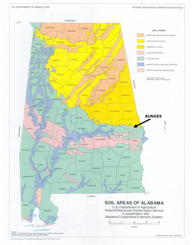
[5] | United States Department of Agriculture (1997) Soil Areas of Alabama, map, USDA NRCS National Cartography and Geospatial Center, Fort Worth, Texas. |
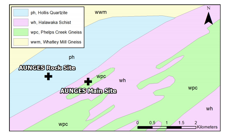
[6] | Yokel LS (1996) Geology of the Chewacla Marble and Associated Units, Lee County, Alabama. Master's Thesis, Auburn University, Auburn, AL. |
[7] | Kahle JK, Brown DA (2002) Performance of Laterally Loaded Drilled Sockets Founded in Weathered Quartzite. Auburn University Highway Research Center, Auburn, Alabama. |
[8] | Szabo MW, Osborne WE, Copeland CW, et al. (1988) Geological Map of Alabama. Special Map 220, Geological Survey of Alabama. |
[9] | Vinson JL, Brown DA (1997) Site Characterization of the Spring Villa Geotechnical Test Site and a Comparison of Strength and Stiffness Parameters for a Piedmont Residual Soil. Report No. IR-97-04, Highway Research Center, Harbert Engineering Center, Auburn University, AL. |
[10] | Mayne PW, Brown DA, Vinson JL, et al. (2000) Site Characterization of Piedmont Residual Soils at the NGES, Opelika, Alabama. National Geotechnical Experimentation Sites, ASCE GSP No. 93, 160–185. |
[11] | Mayne PW, Brown DA (2003) Site Characterization of Piedmont Residuum of North America. Charact Eng Prop Nat Soils 2: 1323–1339. |
[12] | McGillivray AV (2007) Enhanced integration of shear wave velocity profiling in direct-push site characterization systems. Ph.D. Dissertation, Georgia Institute of Technology, Atlanta, GA. |
[13] | Burrage RE (2015) Full Scale Testing of Two Excavations in an Unsaturated Piedmont Residual Soil. Doctoral Disseration, Auburn University. |
[14] | Skinner Z (2019) Theoretical Modeling and Lateral Load Testing of Driven Steel Pile Bridge Bents. Masters's Thesis, Auburn University. |
[15] |
Hebeler GL, Martinez A, Frost JD (2018) Interface Response-Based Soil Classification System. Can Geotech J 55: 1795–1811. doi: 10.1139/cgj-2017-0498
![]() |
[16] | Shi C (2018) Investigation of Deep Foundations at the Spring Villa National Geotechnical Experimentation Site. Master's Thesis, Auburn University. |
[17] | Montgomery J, Shi C, Anderson JB (2018) An Updated Database for the Spring Villa National Geotechnical Experimentation Site. IFCEE 2018: Installation, Testing, and Analysis of Deep Foundations, ASCE GSP No. 294. |
[18] | Brown DA (2002a) The Effect of Construction Technique on Axial Capacity of Drilled Foundations. Auburn University Highway Research Center, Auburn, Alabama. |
[19] | Brown DA (2002b) Report of Statnanic Tests on Rock Sockets at Spring Villa, Alabama. Auburn University Highway Research Center, Auburn, Alabama. |
[20] | Simpson M, Brown DA (2003) Development of P-Y curves for Piedmont residual soils. Auburn University Highway Research Center, Auburn, Alabama. |
[21] | Brown DA (1999) An Experiment with Statnamic Lateral Loading of a Drilled Shaft. Geotechnical Special Publication No. 88: Analysis, Design, Construction and Testing of Deep Foundations, Proceedings of the OTRC '99 Conference, ASCE, 309–318. |
[22] | Brown DA (2019) Personal communication. |
[23] | Robinson B, Rausche F, Likins GE, et al. (2002) Dynamic Load Testing of Drilled Shafts at National Geotechnical Experimentation Sites. Deep Foundations 2002, An International Perspective on Theory, Design, Construction, and Performance, Geotechnical Special Publication No. 116. |
[24] | Brown DA, Drew C (2000) Axial Capacity of Augered Displacement Piles at Auburn University. New Technological and Design Developments in Deep Foundations ASCE GSP No. 100. |
[25] | Brown DA, Nilsson JP (1998) Prefabricated Foundation Elements for Substation Structures. Final Project Report for Alabama Power Co. |
[26] | Brown DA, O'Neill WM, Hoit M, et al. (2001) Static and Dynamic Lateral Loading of Pile Groups. NCHRP 24-9, Transportation Research Board. |
[27] | Brown DA (2002c) Effect of Construction on Axial Capacity of Drilled Foundations in Piedmont Soils. J Geotech Geoenvir Eng 128: 967–973. |
[28] | Brown DA (2007) Rapid Lateral Load Testing of Deep Foundations. DFI 1: 54–62. |
[29] |
Hodgson D, Schindler AK, Brown DA, et al. (2005) Self-consolidating concrete (SCC) for use in drilled shaft applications. J Math Civil Eng 17: 363–369. doi: 10.1061/(ASCE)0899-1561(2005)17:3(363)
![]() |
[30] | Mullins G (2004) Factors Affecting Anomaly Formation in Drilled Shafts-final report. Final Rep. Submitted Florida Department of Transportation, Fla |
[31] | Mullins G, Ashmawy A (2005) Post grouting drilled shaft tips-Phase II final report. Final Rep. Submitted Florida Department of Transportation, Fla |
[32] | Burrage RE, Anderson JB, Pando MA, et al. (2012) A Cost Effective Triaxial Test Method for Unsaturated Soils. Geotech Test J 35: 50–59. |
[33] | Englert CM, Gómez JE, Wilkinson C, et al. (2015) Development of Removable Load Distributive Compressive Anchor Technology. IFCEE 2015, GSP No. 256, ASCE, Reston, VA. |
[34] | Marshall JD, Anderson JB, Campbell J, et al. (2017) Experimental validation of analysis methods and design procedures for steel pile bridge bents. Auburn University Highway Research Center, Auburn, Alabama. |
[35] | Anderson JB, Marshall JD, Campbell J, et al. (2018) Weak axis lateral load testing of a four H pile bent. IFCEE 2018, ASCE GSP 294, 419–427. |
[36] | Anderson JB, Marshall JD (2019) Weak axis lateral load testing of a four vertical H pile bent in residual soil at the Auburn National Geotechnical Experimentation Site. ISGTS 2019. |
[37] | Mayne PW (2000) Seismic Cone Testing at Spring Villa NGES Opelika-Auburn, Alabama. Available from: geosystems.ce.gatech.edu/Faculty/Mayne/Research/summer2000/opelika/opelika.htm. |
[38] | Sowers GF, Richardson TL (1983) Residual Soils of Piedmont and Blue Ridge. Transp Res Rec, 10–16. |
[39] |
Park C, Miller R, Xia J (1999) Multi-channel analysis of surface waves. Geophysics 64: 800–808. doi: 10.1190/1.1444590
![]() |
[40] | Martin GK, Mayne PW (1998) Seismic flat dilatometer tests in Piedmont residual soils. Geotech Site Charact 2: 837–843. |
1. | T Savu, A B Jugravu, Vehicles fleet communications in data infrastructure unavailability situations, 2022, 1268, 1757-8981, 012007, 10.1088/1757-899X/1268/1/012007 | |
2. | Zuoming Zou, Shuming Yang, Liang Zhao, Dual-loop control and state prediction analysis of QUAV trajectory tracking based on biological swarm intelligent optimization algorithm, 2024, 14, 2045-2322, 10.1038/s41598-024-69911-5 | |
3. | Rasmus Dovnborg Frederiksen, Grzegorz Bocewicz, Peter Nielsen, Grzegorz Radzki, Zbigniew Banaszak, A Reference Modelling Approach for Cost Optimal Maintenance for Offshore Wind Farms, 2024, 16, 2071-1050, 8352, 10.3390/su16198352 |
F(θ)=9ms,∀Θ∈[0°,360°) | |||||||||||||||
ILOG | Genetic Algorithm (GA) | ||||||||||||||
C1 | C2 | C3 | |||||||||||||
n | K | TC | fILOG0 | mT | σ | fGA0 | % | mT | σ | fGA0 | % | mT | σ | fGA0 | % |
40 | 2 | 2, 17 | 300 | 60 | 34,214 | 300 | 100 | 0, 06 | 0,015 | 205 | 68, 33 | 58, 51 | 0, 45 | 285 | 95, 00 |
3 | 3, 73 | 450 | 15, 45 | 4,726 | 450 | 100 | 5, 68 | 1,883 | 300 | 66, 67 | 78, 37 | 23,258 | 330 | 73, 33 | |
4 | 151, 69 | 600 | 11, 27 | 4,472 | 600 | 100 | 15, 69 | 0,236 | 355 | 59, 17 | 111, 36 | 1,133 | 420 | 70, 00 | |
60 | 2 | 6, 62 | 300 | 57, 33 | 27, 25 | 300 | 100 | 5, 28 | 1,903 | 240 | 80, 00 | 92, 11 | 0,577 | 285 | 95, 00 |
3 | 34, 25 | 450 | 3, 52 | 8, 94 | 450 | 100 | 9, 78 | 0,264 | 275 | 61, 11 | 142, 55 | 0,618 | 375 | 83, 33 | |
4 | 230 | 600 | 14, 86 | 5,613 | 600 | 100 | 24, 17 | 0,592 | 385 | 64, 17 | 212, 7 | 1,009 | 435 | 72, 50 | |
80 | 2 | 11, 1 | 300 | 68, 7 | 35, 29 | 300 | 100 | 8, 52 | 0,059 | 240 | 80, 00 | 141, 76 | 0,585 | 270 | 90, 00 |
3 | 80 | 450 | 25, 7 | 12, 96 | 450 | 100 | 16, 05 | 0,307 | 355 | 78, 89 | 230, 05 | 0,934 | 390 | 86, 67 | |
4 | 382, 29 | 600 | 20, 97 | 12,468 | 600 | 100 | 34, 66 | 0, 89 | 360 | 60, 00 | 339, 92 | 1,729 | 420 | 70, 00 | |
100 | 2 | 53, 41 | 300 | 23, 03 | 6,041 | 300 | 100 | 12, 39 | 0,064 | 220 | 73, 33 | 212, 62 | 1,625 | 270 | 90, 00 |
3 | 131 | 450 | 31 | 0,407 | 450 | 100 | 23, 68 | 0,435 | 320 | 71, 11 | 318, 17 | 3, 49 | 360 | 80, 00 | |
4 | t>600 | × | 29, 24 | 15,966 | 600 | 100 | 71, 84 | 1,832 | 345 | 57, 50 | 600 | 2,834 | 480 | 80, 00 | |
120 | 2 | 64, 56 | 300 | 70 | 9, 36 | 300 | 100 | 30, 57 | 0,118 | 265 | 88, 33 | 272, 3 | 1,079 | 300 | 100, 00 |
3 | 226, 34 | 450 | 34 | 0,997 | 450 | 100 | 70, 12 | 1,282 | 330 | 73, 33 | 591, 49 | 2,769 | 370 | 82, 22 | |
4 | t>600 | × | 29 | 22,613 | 600 | 100 | 136, 26 | 1,768 | 360 | 60, 00 | t>600 | × | × | × | |
140 | 2 | 136, 67 | 300 | 42 | 17, 73 | 300 | 100 | 65, 05 | 0,059 | 255 | 85, 00 | 495, 11 | 0, 75 | 285 | 95, 00 |
3 | 599, 32 | 450 | 21, 68 | 1, 25 | 450 | 100 | 62, 51 | 1, 03 | 335 | 74, 44 | t>600 | × | × | × | |
4 | t>600 | × | 66, 53 | 26, 45 | 600 | 100 | 143, 45 | 0, 74 | 375 | 62, 50 | t>600 | × | × | × | |
160 | 2 | 368, 99 | 300 | 40, 21 | 22, 58 | 300 | 100 | 43, 19 | 0, 43 | 225 | 75, 00 | 599, 98 | 0, 58 | 300 | 100, 00 |
3 | t>600 | × | 24, 11 | 7, 06 | 450 | 100 | 78, 12 | 1, 01 | 315 | 70, 00 | t>600 | × | × | × | |
4 | t>600 | × | 81 | 37, 04 | 600 | 100 | 180, 77 | 1, 43 | 380 | 63, 33 | t>600 | × | × | × | |
180 | 2 | 415, 55 | 300 | 91 | 15, 15 | 300 | 100 | 54, 27 | 0, 47 | 285 | 95, 00 | t>600 | × | × | × |
3 | t>600 | × | 37 | 12, 55 | 450 | 100 | 103, 34 | 0, 98 | 290 | 64, 44 | t>600 | × | × | × | |
4 | t>600 | × | 119, 66 | 45, 72 | 600 | 100 | 241, 23 | 1, 6 | 375 | 62, 50 | t>600 | × | × | × | |
200 | 2 | 576, 72 | 300 | 65, 66 | 8, 2 | 300 | 100 | 66, 61 | 0, 74 | 250 | 83, 33 | t>600 | × | × | × |
3 | t>600 | × | 38, 7 | 6, 54 | 450 | 100 | 133, 09 | 0, 67 | 305 | 67, 78 | t>600 | × | × | × | |
4 | t>600 | × | 171, 35 | 61, 81 | 600 | 100 | 318, 89 | 1, 7 | 360 | 60, 00 | t>600 | × | × | × | |
220 | 2 | t>600 | × | 79, 22 | 11, 21 | 300 | 100 | 82, 72 | 1, 59 | 225 | 75, 00 | t>600 | × | × | × |
3 | t>600 | × | 49, 89 | 8, 73 | 450 | 100 | 156, 67 | 1, 01 | 290 | 64, 44 | t>600 | × | × | × | |
4 | t>600 | × | 200, 73 | 78, 4 | 600 | 100 | 363, 03 | 1, 65 | 350 | 58, 33 | t>600 | × | × | × | |
Note: n —number of nodes (delivery points); K —size of the UAV fleet; TC —time of computation for IBM ILOG; mT —average calculation time for GA; σ —standard deviation of calculation time; f0 —value of the objective function; %—percentage assessment of the difference between solutions obtained from ILOG and GA: fGA0fILOG0 [%]. |
F(θ)=10ms,∀Θ∈[0°,360°) | |||||||||||||||
ILOG | Genetic Algorithm (GA) | ||||||||||||||
C1 | C2 | C3 | |||||||||||||
n | K | TC | fILOG0 | mT | σ | fGA0 | % | mT | σ | fGA0 | % | mT | σ | fGA0 | % |
40 | 2 | 3,845 | 300 | 48, 2 | 14,928 | 300 | 100 | 3, 26 | 1,592 | 235 | 78, 33 | 47, 85 | 18,871 | 255 | 85, 00 |
3 | 5,131 | 450 | 2, 45 | 3,773 | 450 | 100 | 6, 2 | 1,838 | 275 | 61, 11 | 71, 74 | 18,385 | 390 | 86, 67 | |
4 | 40,021 | 555 | 13, 46 | 34,729 | 600 | 100 | 18, 27 | 0, 51 | 350 | 58, 33 | 107, 18 | 8,773 | 405 | 67, 50 | |
60 | 2 | 7,859 | 300 | 65, 32 | 21,081 | 300 | 100 | 5, 67 | 1,771 | 215 | 71, 67 | 83, 56 | 16, 7 | 270 | 90, 00 |
3 | 28,583 | 450 | 4, 14 | 6,781 | 450 | 100 | 10, 51 | 1,666 | 305 | 67, 78 | 132, 41 | 10,643 | 370 | 82, 22 | |
4 | 394,009 | 600 | 17, 67 | 12,881 | 600 | 100 | 28, 24 | 1,576 | 340 | 56, 67 | 200, 59 | 6,408 | 410 | 68, 33 | |
80 | 2 | 18,647 | 300 | 25 | 3, 83 | 300 | 100 | 9, 13 | 0,614 | 255 | 85, 00 | 135, 9 | 16,463 | 285 | 95, 00 |
3 | 167,592 | 450 | 5, 7 | 4,599 | 450 | 100 | 16, 26 | 0,625 | 310 | 68, 89 | 216, 76 | 7,469 | 400 | 88, 89 | |
4 | t>600 | × | 23, 07 | 6,502 | 600 | 100 | 40, 63 | 0,607 | 350 | 58, 33 | 318, 51 | 1,111 | 370 | 61, 67 | |
100 | 2 | 49,724 | 300 | 3, 04 | 26,858 | 300 | 100 | 12, 5 | 1,027 | 240 | 80, 00 | 197, 63 | 13,839 | 285 | 95, 00 |
3 | 49,194 | 450 | 145 | 10,953 | 450 | 100 | 25, 42 | 1,213 | 295 | 65, 56 | 317, 09 | 1,416 | 355 | 78, 89 | |
4 | t>600 | × | 152 | 12,186 | 600 | 100 | 79, 71 | 1,639 | 375 | 62, 50 | t>600 | × | × | × | |
120 | 2 | 52,216 | 300 | 196 | 0,912 | 300 | 100 | 17, 39 | 1, 71 | 235 | 78, 33 | 271, 71 | 2,794 | 285 | 95, 00 |
3 | t>600 | × | 212 | 8,147 | 450 | 100 | 45, 84 | 0,991 | 310 | 68, 89 | t>600 | × | × | × | |
4 | t>600 | × | 61, 28 | 7,747 | 600 | 100 | 103, 37 | 1,571 | 350 | 58, 33 | t>600 | × | × | × | |
140 | 2 | 131,188 | 300 | 9, 71 | 10,639 | 300 | 100 | 32, 44 | 1,324 | 225 | 75, 00 | 499, 47 | 7,476 | 280 | 93, 33 |
3 | t>600 | 60 | 21, 54 | 3,511 | 450 | 100 | 61, 14 | 0,935 | 315 | 70, 00 | t>600 | × | × | × | |
4 | t>600 | × | 83, 21 | 3,003 | 600 | 100 | 144, 88 | 1,046 | 390 | 65, 00 | t>600 | × | × | × | |
160 | 2 | 356,773 | 300 | 10, 24 | 5,985 | 300 | 100 | 42, 83 | 0,453 | 255 | 85, 00 | t>600 | × | × | × |
3 | t>600 | × | 28, 05 | 4,633 | 450 | 100 | 80, 28 | 1,808 | 315 | 70, 00 | t>600 | × | × | × | |
4 | t>600 | × | 65 | 6,726 | 600 | 100 | 202, 13 | 0,641 | 400 | 66, 67 | t>600 | × | × | × | |
180 | 2 | 541,505 | 300 | 98 | 15,498 | 300 | 100 | 53, 36 | 1,072 | 225 | 75, 00 | t>600 | × | × | × |
3 | t>600 | × | 35, 02 | 8,192 | 450 | 100 | 102, 86 | 0, 62 | 330 | 73, 33 | t>600 | × | × | × | |
4 | t>600 | × | 150, 85 | 8,599 | 600 | 100 | 268 | 1,556 | 365 | 60, 83 | t>600 | × | × | × | |
200 | 2 | 599,257 | 300 | 19, 27 | 0,625 | 300 | 100 | 72, 3 | 1,418 | 245 | 81, 67 | t>600 | × | × | × |
3 | t>600 | × | 44, 91 | 1,009 | 450 | 100 | 135, 6 | 1,036 | 305 | 67, 78 | t>600 | × | × | × | |
4 | t>600 | × | 202, 68 | 1,436 | 600 | 100 | 354, 15 | 1,509 | 365 | 60, 83 | t>600 | × | × | × | |
220 | 2 | t>600 | × | 19, 37 | 0, 54 | 300 | 100 | 81, 89 | 0,754 | 235 | 78, 33 | t>600 | × | × | × |
3 | t>600 | × | 57, 78 | 5,329 | 450 | 100 | 165, 16 | 1,751 | 300 | 66, 67 | t>600 | × | × | × | |
4 | t>600 | × | 239, 33 | 0,801 | 600 | 100 | 428, 7 | 0,626 | 365 | 60, 83 | t>600 | × | × | × | |
Note: n —number of nodes (delivery points); K —size of the UAV fleet; TC – time of computation for IBM ILOG; mT —average calculation time for GA; σ - standard deviation of calculation time; f0 —value of the objective function; % - percentage assessment of the difference between solutions obtained from ILOG and GA: fGA0fILOG0 [%]. |
F(θ)=11ms,∀Θ∈[0°,360°) | |||||||||||||||
ILOG | Genetic Algorithm (GA) | ||||||||||||||
C1 | C2 | C3 | |||||||||||||
n | K | TC | fILOG0 | mT | σ | fGA0 | % | mT | σ | fGA0 | % | mT | σ | fGA0 | % |
40 | 2 | 3,957 | 300 | 96 | 30,905 | 300 | 100 | 3, 53 | 1,058 | 225 | 75, 00 | 47,771 | 21,925 | 270 | 90, 00 |
3 | 5,599 | 450 | 9, 32 | 34,568 | 450 | 100 | 6, 95 | 1,379 | 270 | 60, 00 | 71,685 | 20,719 | 330 | 73, 33 | |
4 | 342,597 | 555 | 19, 72 | 31,304 | 600 | 100 | 24, 3 | 1,781 | 390 | 65, 00 | 112,225 | 16,231 | 390 | 65, 00 | |
60 | 2 | 6,845 | 300 | 32 | 7,138 | 300 | 100 | 6, 11 | 1,083 | 205 | 68, 33 | 83,249 | 21,772 | 255 | 85, 00 |
3 | 12,292 | 450 | 45, 61 | 9,525 | 450 | 100 | 11, 43 | 0,841 | 270 | 60, 00 | 131, 21 | 14,801 | 325 | 72, 22 | |
4 | 29,543 | 600 | 25, 54 | 10,312 | 600 | 100 | 38, 16 | 1,102 | 330 | 55, 00 | 204,368 | 14,424 | 385 | 64, 17 | |
80 | 2 | 14,705 | 300 | 12 | 11,621 | 300 | 100 | 9, 85 | 1,296 | 220 | 73, 33 | 134,987 | 16,747 | 285 | 95, 00 |
3 | 31,342 | 450 | 7, 27 | 6,468 | 450 | 100 | 18, 72 | 1,435 | 285 | 63, 33 | 213,583 | 15,717 | 345 | 76, 67 | |
4 | 464, 70 | × | 32, 29 | 5, 84 | 600 | 100 | 53, 94 | 1, 32 | 365 | 60, 83 | 332, 77 | 21,899 | 440 | 73, 33 | |
100 | 2 | 47,528 | 300 | 3, 73 | 5,277 | 300 | 100 | 14, 25 | 0,485 | 240 | 80, 00 | 196,489 | 5,106 | 285 | 95, 00 |
3 | t>600 | × | 24 | 5,703 | 450 | 100 | 26, 79 | 1,146 | 300 | 66, 67 | 320,935 | 17,292 | 405 | 90, 00 | |
4 | t>600 | × | 36 | 5,605 | 600 | 100 | 105, 38 | 1,101 | 350 | 58, 33 | t>600 | × | × | × | |
120 | 2 | 69,069 | 300 | 58 | 12,056 | 300 | 100 | 20, 05 | 1,357 | 250 | 83, 33 | 272,852 | 22,023 | 285 | 95, 00 |
3 | 271, 93 | 450 | 18, 2 | 5,425 | 450 | 100 | 47, 08 | 1, 23 | 305 | 67, 78 | 595,066 | 20,186 | 360 | 80, 00 | |
4 | 486,909 | 600 | 35 | 1,515 | 600 | 100 | 119, 51 | 1,746 | 365 | 60, 83 | t>600 | × | × | × | |
140 | 2 | 93,477 | 300 | 98 | 8,019 | 300 | 100 | 33, 55 | 1,701 | 225 | 75, 00 | 493,384 | 5,415 | 270 | 90, 00 |
3 | 476, 9 | 450 | 24, 52 | 5,884 | 450 | 100 | 62, 62 | 1,753 | 310 | 68, 89 | t>600 | × | × | × | |
4 | 578,965 | 600 | 118, 43 | 3,601 | 600 | 100 | 164, 53 | 1,592 | 340 | 56, 67 | t>600 | × | × | × | |
160 | 2 | 155,018 | 300 | 12, 71 | 6,243 | 300 | 100 | 43, 23 | 1,808 | 235 | 78, 33 | t>600 | × | × | × |
3 | t>600 | × | 32, 04 | 1,503 | 450 | 100 | 85, 6 | 0,579 | 295 | 65, 56 | t>600 | × | × | × | |
4 | t>600 | × | 154 | 5,646 | 600 | 100 | 226, 91 | 1,781 | 370 | 61, 67 | t>600 | × | × | × | |
180 | 2 | 351,507 | 300 | 222 | 30,871 | 300 | 100 | 53, 73 | 0,867 | 220 | 73, 33 | t>600 | × | × | × |
3 | t>600 | × | 40, 46 | 3,673 | 450 | 100 | 102, 23 | 0,861 | 285 | 63, 33 | t>600 | × | × | × | |
4 | t>600 | × | 193, 15 | 18,532 | 600 | 100 | 292, 14 | 1,027 | 410 | 68, 33 | t>600 | × | × | × | |
200 | 2 | 584,659 | 300 | 50 | 0,621 | 300 | 100 | 66, 79 | 1,518 | 220 | 73, 33 | t>600 | × | × | × |
3 | t>600 | × | 48 | 1,259 | 450 | 100 | 129, 77 | 1,351 | 330 | 73, 33 | t>600 | × | × | × | |
4 | t>600 | × | 281, 58 | 1,426 | 600 | 100 | 420, 34 | 0, 77 | 345 | 57, 50 | t>600 | × | × | × | |
220 | 2 | t>600 | × | 23, 56 | 0, 7 | 300 | 100 | 82, 01 | 1,361 | 220 | 73, 33 | t>600 | × | × | × |
3 | t>600 | × | 65, 46 | 1,086 | 450 | 100 | 167, 36 | 0,671 | 310 | 68, 89 | t>600 | × | × | × | |
4 | t>600 | × | 331, 64 | 1,112 | 600 | 100 | 485, 18 | 0,854 | 365 | 60, 83 | t>600 | × | × | × | |
Note: n —number of nodes (delivery points); K – size of the UAV fleet; TC —ime of computation for IBM ILOG; mT —average calculation time for GA; σ —standard deviation of calculation time; f0 —value of the objective function; %—percentage assessment of the difference between solutions obtained from ILOG and GA: fGA0fILOG0 [%]. |