Bifurcation and chaos in N-type and S-type muscular blood vessel models

Wenxin Zhang; Lijun Pei; Wenxin Zhang; Lijun Pei

doi:10.3934/era.2025057

Electronic Research Archive

2025, Volume 33, Issue 3: 1285-1305. doi: 10.3934/era.2025057

Previous Article Next Article

Research article Special Issues

Bifurcation and chaos in N-type and S-type muscular blood vessel models

Wenxin Zhang ,
Lijun Pei ^,

School of Mathematics and Statistics, Zhengzhou University, Zhengzhou 450001, China

Received: 06 November 2024 Revised: 31 January 2025 Accepted: 07 February 2025 Published: 04 March 2025

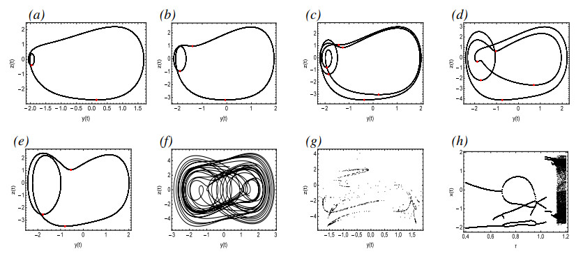
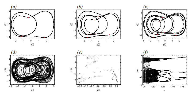
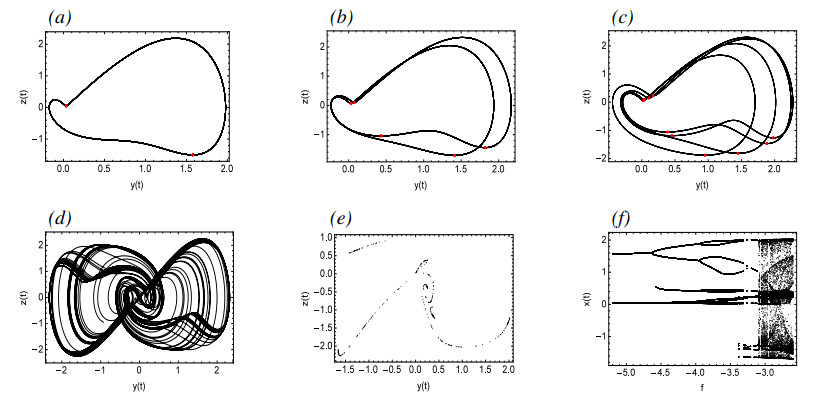
In this paper, we have constructed two muscular blood vessel systems influenced by external disturbances by using the non-autonomous delayed differential equation (DDE). As an important physiological structure of the human body, muscle blood vessels participate in many activities such as blood flow. Many diseases are associated with abnormal dynamics of muscle blood vessels. From a mathematical point of view, vasospasm is caused by a chaotic state of blood vessels. Vasospasm is the manifestation of this disease in the vascular system, which can cause blood vessel blockage and even harm human health when it is serious. We conducted the dynamical analysis of the S-type and N-type muscular blood vessel systems by utilizing bifurcation diagrams, time histories, and pseudo-phase portraits, and investigated the effects of different parameters on these systems. Specifically, when parameters change, rich dynamical phenomena occur, such as equilibria, periodic solutions, quasi-periodic solutions, Hopf bifurcation, and chaos, as well as the route of period-doubling bifurcation to chaos. Meanwhile, we analyzed approximate analytical solutions by using the method of multiple scales (MMS) and determined the stability of steady-state solutions through the Routh-Hurwitz criterion. The results indicate that the MMS can deduce better analytical results for some non-autonomous DDEs.

Keywords:

Citation: Wenxin Zhang, Lijun Pei. Bifurcation and chaos in N-type and S-type muscular blood vessel models[J]. Electronic Research Archive, 2025, 33(3): 1285-1305. doi: 10.3934/era.2025057

Related Papers:

[1]	Junhai Ma, Hui Jiang . Dynamics of a nonlinear differential advertising model with single parameter sales promotion strategy. Electronic Research Archive, 2022, 30(4): 1142-1157. doi: 10.3934/era.2022061
[2]	Danyang Wang, Ning Chen . Research on Hopf bifurcation of vehicle air compressor system with single-pendulum TMD. Electronic Research Archive, 2025, 33(5): 3285-3304. doi: 10.3934/era.2025145
[3]	Yang Jin, Wanxiang Li, Hongbing Zhang . Transition characteristics of the dynamic behavior of a vehicle wheel-rail vibro-impact system. Electronic Research Archive, 2023, 31(11): 7040-7060. doi: 10.3934/era.2023357
[4]	Jiange Dong, Xianyi Li . Bifurcation of a discrete predator-prey model with increasing functional response and constant-yield prey harvesting. Electronic Research Archive, 2022, 30(10): 3930-3948. doi: 10.3934/era.2022200
[5]	Qinghua Zhu, Meng Li, Fang Han . Hopf bifurcation control of the ML neuron model with Hc bifurcation type. Electronic Research Archive, 2022, 30(2): 615-632. doi: 10.3934/era.2022032
[6]	Qixiang Wen, Shenquan Liu, Bo Lu . Firing patterns and bifurcation analysis of neurons under electromagnetic induction. Electronic Research Archive, 2021, 29(5): 3205-3226. doi: 10.3934/era.2021034
[7]	Zhili Zhang, Aying Wan, Hongyan Lin . Spatiotemporal patterns and multiple bifurcations of a reaction- diffusion model for hair follicle spacing. Electronic Research Archive, 2023, 31(4): 1922-1947. doi: 10.3934/era.2023099
[8]	Leiting Wang, Yang Jin, Wangxiang Li, Chenyang Tang . Analysis of the nonlinear dynamic behavior of longitudinal systems in heavy-haul trains. Electronic Research Archive, 2025, 33(2): 582-599. doi: 10.3934/era.2025027
[9]	Mengting Sui, Yanfei Du . Bifurcations, stability switches and chaos in a diffusive predator-prey model with fear response delay. Electronic Research Archive, 2023, 31(9): 5124-5150. doi: 10.3934/era.2023262
[10]	Yanlong Zhang, Rui Zhang, Li Wang . Oblique impact dynamic analysis of wedge friction damper with Dankowicz dynamic friction. Electronic Research Archive, 2024, 32(2): 962-978. doi: 10.3934/era.2024047

Abstract

1. Introduction

In the human body, the heart controls the flow of blood through various blood vessels. Blood vessels are divided into arteries, capillaries, and veins according to their functions. Arteries transport fresh oxygen from the heart to all tissues in the body. The coronary artery system is composed of two blood vessels that diverge from the aorta. They are very close to the starting point of the heart. According to reports, coronary artery disease is the leading global cause of mortality and morbidity ^[1,2,3]. Unfortunately, accurate prediction and assessment of mortality or morbidity remains difficult due to the complexity of the interdependence of various factors and the ambiguity of the data. Compared with the traditional binary logistic regression model to predict the mortality after coronary artery bypass surgery, the fuzzy expert system introduced by Nouei et al. can greatly improve the classification accuracy ^[4]. Auffret et al. discussed the incidence, prognostic impact, and unmet needs of patients with new conduction disorders after transcatheter aortic valve replacement, as well as the ongoing challenges associated with the management of concomitant coronary artery disease ^[5]. Coronary angiography is the process of using X-rays to determine and observe the heart condition. It is the main imaging technique for diagnosing coronary diseases and is the standard for evaluating clinically significant coronary artery disease ^[6,7,8,9]. The 3D reconstruction of rotational coronary angiography can provide the required information volume for clinical applications ^[10]. Automatic 3D blood vessel reconstruction to improve vascular diagnosis and treatment is a challenging task, where real-time implementation of automatic segmentation and specific vascular tracking for matching artery sequences are essential ^[11,12]. Since most of the vascular interventional robots cannot cope with the complicated coronary artery lesions in clinical practice, the risk of surgery will be increased. Yu et al. developed a vascular interventional robot that can accurately measure the delivery resistance of interventional instruments and provide tactile force feedback to doctors ^[13].

As we all know, more and more attention has been paid to non-autonomous dynamical systems in various fields of research, including ecology (such as describing the growth and competition relationships of biological populations), economics (such as describing the delayed response to market demand), and control theory (such as describing control systems with time-varying characteristics and delayed feedback). In practical applications, non-autonomous delayed differential equations can help us to understand and predict the dynamical behavior of the system more accurately. Non-autonomous differential equations can also be used to describe multi-agent systems and design corresponding control protocols ^[14,15]. The profound discussion of the coronary artery system as a practical biological mathematical case of the non-autonomous system is of great significance. The dynamics of a two-dimensional non-autonomous coronary artery model is investigated. Numerical simulations show that the system exhibits chaotic attractors, quasi-periodic attractors, and periodic orbits. For some specific parameter sets, two different solutions appear, and these coexisting attractors exhibit different complexity. It indicates that the dynamical characteristics of the coronary artery system are difficult to predict ^[16]. Many medical experts have concluded that vasospasm is the main cause of myocardial ischemia and other cardiovascular diseases, such as common angina pectoris, sudden death, myocardial infarction, etc. From the mathematical perspective, vascular spasm is caused by the chaotic state of blood vessels ^[17,18,19]. Singh et al. suggested that the chaotic states of abnormal vasospasm in blood vessels make heart disease patients more susceptible to severe COVID-19 infections, ultimately leading to high mortality rates ^[20].

Bifurcation is always an important topic in nonlinear dynamics research ^[21], which can lead to some complex dynamical phenomena. The Hopf bifurcation is an important research area of non-autonomous delayed differential equations in the field of nonlinear dynamics, which has been widely applied to biology, physics, economics, and so on. However, the Hopf bifurcation of non-autonomous systems is very difficult to predict even in deterministic conditions. As a result, there are not many theories on it. Due to the sensitivity to disturbances, abnormal and fatal chaos in the system can induce coronary artery disease. In view of the signification of the dynamics of the coronary artery system, extensive researches have been conducted on it. By designing a chaotic observer and constructing a Lyapunov-Krasovskii functional (LKF) for the master-slave system, a more conservative synchronization strategy was obtained for chaotic coronary artery systems with state estimation errors and synchronization errors ^[22]. Ding et al. utilized disturbance observer technology to discuss the chaotic suppression of the coronary artery system, and designed a smooth second-order sliding mode controller to suppress the chaos of the coronary artery system ^[23]. Chantawat and Botmart were the first to investigate the finite-time H-infinity synchronization control for the coronary artery chaotic system with input and state time-varying delays ^[24]. They designed a synchronous feedback controller with good performance in the presence of disturbance and time-varying delay. This synchronization strategy can effectively synchronize the convulsive coronary artery system with the healthy cardiovascular system. From an engineering perspective, Qian et al. adopted a combination of the derivative-integral terminal sliding mode controller and disturbance observer to suppress chaos ^[25]. The simulation results verified the effectiveness of the proposed strategy. The adaptive feedback scheme combining linear state feedback and adaptive laws can also lead an abnormal muscular blood vessel to a normal track ^[26]. The coronary artery system is a complex biological system. Their chaotic phenomenon can lead to serious health problems. In order to suppress chaotic phenomena, various control methods have been proposed, such as an adaptive observer ^[27], self-tuning integral-type finite-time-stabilized sliding mode control ^[28], synchronization controller ^[29], generalized dissipative control method ^[30], terminal sliding mode control with self-tuning ^[31], etc. In fact, most of these researches involve suppressing chaos or synchronizing hemodynamics in the coronary artery system. However, there are not many explorations on the dynamics of coronary artery systems with periodic disturbances under certain parameter changes. Therefore, further researches on this system is of great significance.

As an important physiological structure in the human body, muscular blood vessels are involved in many aspects such as blood flow. Many diseases, such as angina pectoris and myocardial infarction, are associated with abnormal dynamics of muscular blood vessels. By studying the dynamical phenomena of muscular blood vessel models, we can explore the cause and development of these diseases, and provide new ideas and methods for disease prevention and treatment. From the mathematical perspective, vascular spasm is caused by the chaotic state of blood vessels. Chaos shows that under certain conditions, the system suddenly deviates from the expected regularity and becomes disordered. Vasospasm is the manifestation of this disorder in the vascular system, which can cause blood vessel blockage in serious cases, thus endangering human health. So through the analysis of dynamical phenomena, we can deepen our understanding of these physiological mechanisms, more accurately diagnose related diseases, and make more effective treatment plans.

The structure of this article is outlined as follows. In Section 2, we introduce the model of the S-type muscular blood vessel. In Section 3, we discuss its steady-state equations. Then we utilize recurrence plots to further validate the dynamics for different parameters ^[32,33]. Finally, bifurcation, chaos, and their numerical verifications are presented. In Section 4, we introduce the model of the N-type muscular blood vessel and obtain its bifurcation diagram from periodic to chaotic motions under different parameter changes. Section 5 presents a brief conclusion.

2. The model of the S-type muscular blood vessel

The model of the S-type muscular blood vessel is denoted as ^[34]

$\begin{equation} { } \left\{ \begin{array}{lr} {\frac{d x}{d t}} = \lambda(y+x-x^3+ {\frac{d y}{d t}}), \\[0.3cm] {\frac{d y}{d t}} = -cx-by.\\[0.3cm] \end{array} \right. \end{equation}$

(2.1)

The system can be considered as

$\begin{equation} { } \begin{array}{l} {\frac{d^2 y}{d t^2}}+(c\lambda-b\lambda)y(t)-(\lambda-c\lambda-b) {\frac{d y}{d t}}+\frac{\lambda b^3}{c^2}y(t)^3+\frac{\lambda}{c^2}( {\frac{d y}{d t}})^3+\frac{3b\lambda}{c^2}y(t)( {\frac{d y}{d t}})^2+\frac{3\lambda b^2}{c^2}y(t)^2 {\frac{d y}{d t}} = 0. \end{array} \end{equation}$

(2.2)

By introducing periodic disturbance and delay, System (2.2) becomes

$\begin{equation} { } \begin{array}{l} {\frac{d^2 y}{d t^2}}+(c\lambda-b\lambda)y(t)-\mu(\lambda-c\lambda-b) {\frac{d y}{d t}}+\mu\frac{\lambda b^3}{c^2}y(t)^3+\mu\frac{\lambda}{c^2}( {\frac{d y}{d t}})^3+\mu\frac{3b\lambda}{c^2}y(t)( {\frac{d y}{d t}})^2+\mu\frac{3\lambda b^2}{c^2}y(t)^2 {\frac{d y}{d t}}\\[0.2cm]-\varepsilon\gamma \cos(\Omega t)y(t-\tau) = 0, \end{array} \end{equation}$

(2.3)

where $y$ is the change of the internal diameter of the vessel, $x$ is the change of the internal pressure of the vessel and the time lag term is considered as a possible backflow caused by the vascular blockage, and $\varepsilon \gamma cos(\Omega t)y(t-\tau)$ is a combination of periodic stimulating disturbances with the time-delayed variation in the vessel internal diameter.

3. Steady-state approximate solution

3.1. MMS

The parameters of Eq (2.3) are suitably scaled as $\mu = \epsilon \hat{\mu}, \varepsilon = \epsilon \hat{\varepsilon}$ . In order to obtain an approximate solution of Eq (2.3), we utilize the method of multiple scales to seek the solution in the following form:

$\begin{equation} { } \left\{ \begin{array}{lr} y(t, \epsilon) = y_0 (T_{0}, T_{1})+\epsilon y_1 (T_{0}, T_{1})+O(\epsilon^2), \\[0.3cm] y(t-\tau, \epsilon) = y_{\tau0} (T_{0}, T_{1})+\epsilon y_{\tau1} (T_{0}, T_{1})+O(\epsilon^2), \end{array} \right. \end{equation}$

(3.1)

where $T_{0} = t$ and $T_{1} = \epsilon t$ are two time scales. The derivatives can be written as follows:

$\begin{equation} { } \frac{d y}{d t} = \frac{\partial y}{\partial T_{0}}+\epsilon \frac{\partial y}{\partial T_{1}}+O(\epsilon^2), \; \; \frac{d^{2} y}{d t^{2}} = \frac{\partial^{2} y}{\partial T_{0}^{2}}+2\epsilon \frac{\partial^{2} y}{\partial T_{0}\partial T_{1}}+O(\epsilon^2). \end{equation}$

(3.2)

Substituting Eqs (3.1) and (3.2) into Eq (2.3), then equating the coefficients of like powers of $\epsilon$ , we obtain the following two differential equations,

$O(\epsilon^{0})$ :

$\begin{equation} { } \frac{\partial^{2}}{\partial T_{0}^{2}} y_0+(c\lambda-b\lambda) y_0 = 0, \\[0.2cm] \end{equation}$

(3.3)

$O(\epsilon^{1})$ :

$\begin{equation} { } \begin{array}{ll} {\frac{\partial^{2}}{\partial T_{0}^{2}}} y_1+\left(c\lambda-b\lambda\right) y_1 = -\hat{\mu}\frac{\lambda b^3}{c^2}y_0^3+\gamma\hat{\varepsilon}\cos(\Omega t)y_{\tau0}-\hat{\mu}\left(-\lambda+c\lambda+b\right)\frac{\partial}{\partial T_{0}}y_0-\hat{\mu} {\frac{3\lambda b^2}{c^2}}y_0^2\frac{\partial}{\partial T_{0}} y_0\\[0.2cm] \ \ \ \ \ \ \ \ \ \ \ \ \ \ \ \ \ \ \ \ \ \ \ \ \ \ \ \ \ \ -\hat{\mu}\frac{3b\lambda}{c^2}y_0\left(\frac{\partial y_0}{\partial T_{0}}\right)^2-\hat{\mu}\frac{\lambda}{c^2}\left(\frac{\partial y_0}{\partial T_{0}}\right)^3-2\frac{\partial^{2}y_0}{\partial T_{0}\partial T_{1}}. \end{array} \end{equation}$

(3.4)

The solution for Eq (3.3) can be represented as

$\begin{equation} { } \begin{array}{l} y_0 (T_{0}, T_{1}) = A(T_1)e^{i\omega T_0}+\bar{A}(T_{1})e^{-i\omega T_0}. \end{array} \end{equation}$

(3.5)

The corresponding time-delayed solutions can be formulated as follows:

$\begin{equation} { } \begin{split} y_{\tau0} (T_{0}, T_{1})& = A(T_1-\epsilon\tau)e^{i\omega (T_0-\tau)}+ \bar{A}(T_1-\epsilon\tau)e^{-i\omega (T_0-\tau)}, \end{split} \end{equation}$

(3.6)

where over-bars represent the complex conjugate. Expanding $A(T_1-\epsilon\tau)$ in the Taylor series yields

$\begin{equation} { } \begin{array}{lr} A(T_1-\epsilon\tau) = A(T_1)-\epsilon\tau A'(T_1)+\frac{(\epsilon\tau_{1})^{2}}{2!}A''(T_1)-\frac{(\epsilon\tau)^{3}}{3!}A'''(T_1)+\cdot\cdot\cdot = A(T_1)+O(\epsilon).\\[0.2cm] \end{array} \end{equation}$

(3.7)

Substituting Eq (3.7) into Eq (3.6) and by retaining only the first terms as approximations, therefore

$\begin{equation} { } \begin{array}{l} y_{\tau_0} (T_{0}, T_{1})\cong A(T_1)e^{i\omega (T_0-\tau)}+\bar{A}(T_1)e^{-i\omega (T_0-\tau)}. \end{array} \end{equation}$

(3.8)

Substituting Eqs (3.5) and (3.6) into Eq (3.4) and taking Eq (3.8) into account, it follows that

$\begin{equation} { } \begin{array}{l} \frac{\partial^{2}}{\partial T_{0}^{2}} y_1+(c\lambda-b\lambda) y_1 = -\Big(\frac{b^{3}\lambda\hat{\mu}(e^{iT_{0}\omega}A+e^{-iT_{0}\omega}\bar{A})^3}{c^2}-\gamma\hat{\varepsilon}\cos(\Omega t)(e^{i(T_{0}-\tau)\omega}A+e^{-i(T_{0}-\tau)\omega}\bar{A})+(b-\lambda+c\lambda)\\[0.2cm]\ \ \ \ \ \ \ \ \ \ \ \ \ \ \ \ \ \ \ \ \ \ \ \ \ \ \ \ \ \ \;\;\times\; \hat{\mu}(ie^{iT_{0}\omega}\omega A-ie^{-iT_{0}\omega}\omega\bar{A}) +\frac{3b^{2}\lambda\hat{\mu}(e^{iT_{0}\omega}A+e^{-iT_{0}\omega}\bar{A})^2(ie^{iT_{0}\omega}\omega A-ie^{-iT_{0}\omega}\omega\bar{A})}{c^2}+\\[0.2cm]\ \ \ \ \ \ \ \ \ \ \ \ \ \ \ \ \ \ \ \ \ \ \ \ \ \ \ \ \ \ \;\;\frac{\lambda\hat{\mu}(ie^{iT_{0}\omega}\omega A-ie^{-iT_{0}\omega}\omega\bar{A})^3}{c^2}+ 2(ie^{iT_{0}\omega} \times\omega A'-ie^{-iT_{0}\omega}\omega \bar{A}')\\[0.2cm]\ \ \ \ \ \ \ \ \ \ \ \ \ \ \ \ \ \ \ \ \ \ \ \ \ \ \ \ \ \ \;\; +\frac{3b\lambda\hat{\mu}(e^{iT_{0}\omega}A+e^{-iT_{0}\omega}\bar{A})(ie^{iT_{0}\omega}\omega A-ie^{-iT_{0}\omega}\omega\bar{A})^2}{c^2}\Big). \end{array} \end{equation}$

(3.9)

Since Eq (3.5) is the solution of Eq (3.3), we have $\omega = \sqrt{c\lambda-b\lambda}$ . The resonance here is 2:1 resonance, i.e., $(\Omega = 2\omega)$ . Substituting (3.5) and (3.8) into (3.4), and utilizing the solvability conditions using the original time scale (i.e., $\hat{\mu} = \frac{\mu}{\epsilon}, \hat{\varepsilon} = \frac{\varepsilon}{\epsilon}$ ), it follows that

$\begin{equation} { } \begin{array}{l} -\frac{1}{2}e^{i\omega\tau}\gamma\varepsilon \bar{A}+ib\mu\omega A-i\lambda\mu\omega A+ic\lambda\mu\omega A+\frac{3b^3\lambda\mu}{c^2}A^2\bar{A}+\frac{3ib^2\lambda\mu\omega}{c^2}A^2\bar{A}+\frac{3b\lambda\mu\omega^2}{c^2}A^2\bar{A} +\frac{3i\lambda\mu\omega^3}{c^2}A^2\bar{A}+2i\omega A' = 0. \end{array} \end{equation}$

(3.10)

Expressing $A$ in terms of the polar form, it follows that

$\begin{equation} { } \left\{ \begin{array}{lr} A = \frac{a}{2}e^{i\phi}\Rightarrow \dot{A} = \frac{\dot{a}}{2}e^{i\phi}+i\frac{a}{2}\dot{\phi} e^{i\phi}, \\[0.2cm] \bar{A} = \frac{a}{2}e^{-i\phi}\Rightarrow \dot{\bar{A}} = \frac{\dot{a}}{2}e^{-i\phi}-i\frac{a}{2}\dot{\phi} e^{-i\phi}, \end{array} \right. \end{equation}$

(3.11)

in the equation, $a$ is the amplitude and $\phi$ is the phases of System (2.3). Substituting Eq (3.11) into Eq (3.10) and equating the real parts of the equation to each other and separately equating the imaginary parts, we get the following equations:

$\begin{equation} { } \left\{ \begin{array}{lr} \dot{a} = \frac{a}{8c^2\omega}\left(-3\lambda\mu\omega\left(b^2+\omega^2\right)a^2+2c^2\left(-2\left(b+\left(-1+c\right)\lambda\right)\mu\omega+\gamma\varepsilon\sin(\omega\tau-2\phi) \right)\right), \\[0.2cm] \dot{\phi} = \frac{1}{8c^2\omega}\left(3b\lambda\mu\left(b^2+\omega^2\right)a^2-2c^2\gamma\varepsilon\cos(\omega\tau-2\phi)\right). \end{array} \right. \end{equation}$

(3.12)

3.2. Stability determination

In the steady state, there exists

$\begin{equation} { } \begin{array}{l} \dot{a} = \dot{\phi} = 0. \end{array} \end{equation}$

(3.13)

From Eq (3.12), it follows that

$\begin{equation} { } \left\{ \begin{array}{lr} \frac{a}{8c^2\omega}\left(-3\lambda\mu\omega\left(b^2+\omega^2\right)a^2+2c^2\left(-2\left(b+\left(-1+c\right)\lambda\right)\mu\omega+\gamma\varepsilon\sin(\omega\tau-2\phi) \right)\right) = 0, \\ \frac{1}{8c^2\omega}\left(3b\lambda\mu\left(b^2+\omega^2\right)a^2-2c^2\gamma\varepsilon\cos(\omega\tau-2\phi)\right) = 0. \end{array} \right. \end{equation}$

(3.14)

The steady-state solution of Eq (3.14) can be numerically obtained via the software MATHEMATICA. In order to analyze the stability of the solution, we can let

$\begin{equation} { } a = a_{0}+a_{1}, \ \ \; \phi = \phi_{0}+\phi_{1}, \end{equation}$

(3.15)

where $a_{0}, \phi_{0}$ satisfy Eq (3.14), and $a_{1}, \phi_{1}$ are small-valued perturbations compared to $a_{0}, \phi_{0}$ . Inserting Eq (3.15) into Eq (3.12) and linearizing it at $(a_{0}, \phi_{0})$ , we get the following linear dynamical system:

$\begin{equation} { } \left({\begin{array}{cc}\dot{a}_{1}\\\dot{\phi}_{1}\\\end{array}}\right) = [J]\left({\begin{array}{cc}a_{1}\\ \phi_{1}\\\end{array}}\right) = \left({\begin{array}{cc}r_{11}&r_{12}\\r_{21}&r_{22}\\\end{array}}\right)\left({\begin{array}{cc}a_{1}\\ \phi_{1}\\\end{array}}\right), \end{equation}$

(3.16)

where $[J] = \left({\begin{array}{cc}r_{11}&r_{12}\\r_{21}&r_{22}\\\end{array}}\right)$ is the Jacobian matrix. The characteristic equation reads as

$\begin{equation} { } \lambda^{2}+\eta_{1}\lambda+\eta_{0} = 0. \end{equation}$

(3.17)

The steady-state solution is asymptotically stable if and only if the real parts of all the eigenvalues $\lambda$ are negative. According to the Routh-Hurwitz criterion, the sufficient and necessary conditions for ensuring that all roots of Eq (3.17) possess negative real parts is

$\begin{equation} { } \eta_{1} > 0, \; \; \eta_{0} > 0. \end{equation}$

(3.18)

3.3. Hopf bifurcation and chaos

Within this subsection, the bifurcation diagrams are produced on the basis of Eq (3.14). Analysis is introduced by using the following values of the system parameters: $\mu = 1, \; \varepsilon = 1, \; c = 1.6, \; b = -1, \; \lambda = 1.6, \; \tau = 1, \; \omega = \sqrt{2.6}, \; \gamma = 0.9$ , unless otherwise stated.

are the $\gamma$ -amplitude curves of approximate solutions by MMS, while compares the approximate analytical solution derived by using MMS with numerical simulation results. The figure reveals that as $\gamma$ decreases gradually, the amplitude of periodic oscillations decreases accordingly. Until point A is reached, where the periodic oscillations cease to exist, this leaves only one unstable equilibrium in the system. From , it is evident that the system exhibits a periodic solution for $\gamma = 0.67$ , and there exists a phase-locked solution for $\gamma = 0.66$ . As $\gamma$ gradually decreases, it can be seen from that for $\gamma = 0.4$ , the system exhibits a quasi-periodic solution. Figure 2(i) presents the process from periodic to quasi-periodic solutions.

Figure 1. (a) The

$\gamma$ -amplitude response curves of the approximate solutions of System (2.3) for

$\lambda = 1$ ; (b) Comparisons between the approximate analytical solution derived using MMS and the numerical simulation results. Red dots: numerical solutions, solid lines: stable solutions, dashed lines: unstable solutions.

DownLoad: Full-Size Img PowerPoint

Figure 2. The evolution of System (2.3) for

$\lambda = 1$ with initial functions with

$y(0) = y(-\tau) = z(0) = z(-\tau) = 0.1$ , where

$z(t) = \dot{y}(t)$ . (a),(b)

$\gamma = 0.67$ ; (c),(d)

$\gamma = 0.66$ ; (e) Poincar

$\acute{\mathrm{e}}$ section with section

$\dot{z} = 0.5$ for

$\gamma = 0.66$ ; (f),(g)

$\gamma = 0.4$ ; (h) Poincar

$\acute{\mathrm{e}}$ section with section

$\dot{z} = 0.5$ for

$\gamma = 0.4$ ; (i) the process of System (2.3) from periodic to quasi-periodic solutions.

DownLoad: Full-Size Img PowerPoint

depicts a bifurcation diagram, where $\lambda$ serves as the primary bifurcation parameter. As $\lambda$ is decreased gradually, prior to reaching point A, System (2.3) possesses a single asymptotically stable equilibrium. However, at point A, a supercritical bifurcation takes place. Subsequent to this bifurcation, there is a stable periodic solution that is marked with a solid line and an unstable equilibrium marked with dashed lines. demonstrate the time history and pseudo-phase portrait for $\lambda = 2.03$ , respectively, revealing the presence of a single asymptotically stable equilibrium at this stage. Following a supercritical Hopf bifurcation, illustrate the time history and pseudo-phase portrait of System (2.3) at $\lambda = 1.98$ , indicating that System (2.3) possesses a stable periodic solution. Then the small-amplitude periodic solutions increase at a remarkable rate from Point A to Point B where the stable periodic solution disappears. reveals that System (2.3) may enter into a chaotic state for $\lambda = 0.6$ . shows the process of System (2.3) from periodic to chaotic motion when $\lambda$ decreases from $0.73$ to $0.6$ . describes the recurrence plots for $\lambda = 0.6$ and $\lambda = 1.98$ . Generally speaking, when the recurrence plot presents a periodic shape, it reflects that the system is in a periodic state. When there are line segments parallel to the main diagonal and separate points mixed together, it is in a chaotic state. It can also be inferred from the figure that it is a periodic solution for $\lambda = 1.98$ , while it has chaotic motions for $\lambda = 0.6$ .

Figure 3. (a) The

$\lambda$ -amplitude response curves of the approximate solutions of System (2.3) for

$\omega = \sqrt{2.6\lambda}$ ; (b) Comparisons between the approximate analytical solution derived using MMS and the numerical simulation results. Red dots: numerical solutions, solid lines: stable solutions, dashed lines: unstable solutions.

DownLoad: Full-Size Img PowerPoint

Figure 4. The numerical simulations of System (2.3) with the initial functions with

$x(0) = x(-\tau) = y(0) = y(-\tau) = 0.1$ , where

$z(t) = \dot{y}(t)$ . (a), (b)

$\lambda = 2.03$ ; (c), (d)

$\lambda = 1.98$ ; (e)

$\lambda = 0.6$ ; (f) the process of System (2.3) from periodic to chaotic motions.

DownLoad: Full-Size Img PowerPoint

Figure 5. Recurrence plots of (a) a periodic motion for

$\lambda = 1.98$ , (b) the chaotic motion for

$\lambda = 0.6$ .

DownLoad: Full-Size Img PowerPoint

illustrates the dynamical phenomena of System (2.3) with the change of parameter $c$ , along with a comparison between the approximate analytical solution obtained through MMS and the numerical simulation results. It can be observed that as the parameter $c$ gradually decreases to point A, a supercritical Hopf bifurcation takes place, resulting in the bifurcation from the asymptotically stable equilibrium to a stable periodic solution and an unstable equilibrium.

Figure 6. (a) The

$c$ -amplitude response curves of the approximate solutions of System (2.3) for

$\omega = \sqrt{1.6(c+1)}$ ; (b) Comparisons between the approximate analytical solution derived using MMS and the numerical simulation results. Red dots: numerical solutions, solid lines: stable solutions, dashed lines: unstable solutions.

DownLoad: Full-Size Img PowerPoint

The numerical simulation presented in describes that $c = 1.77$ before the bifurcation is an asymptotically stable equilibrium, as shown in . After the bifurcation Point A, for $c = 1.75$ , there is a stable periodic solution as represented in . As $c$ continues to decrease, the amplitude of the periodic solution continuously increases until it reaches Point B. Subsequent to Point B, the periodic solution disappears, and as presented in –, the quasi-periodic solution appears for $c = 1.29$ .

Figure 7. The numerical simulations of System (2.3) with the initial functions with

$x(0) = x(-\tau) = y(0) = y(-\tau) = 0.1$ , where

$z(t) = \dot{y}(t)$ . (a), (b)

$c = 1.75$ ; (c), (d)

$c = 1.77$ ; (e), (f)

$c = 1.29$ ; (g) Poincar

$\acute{\mathrm{e}}$ section with section

$\dot{z} = 0.6$ for

$c = 1.29$ ; (h) the process of System (2.3) from periodic to quasi-periodic solutions.

DownLoad: Full-Size Img PowerPoint

As shown in , supercritical Hopf bifurcation will occur at Point A and produce a stable periodic solution, but as $b$ gradually decreases, the stable periodic solution disappears at Point B. From Figure 8(b), it can be seen that the approximate analytical solution obtained by MMS is in good agreement with the numerical simulation results, indicating the effectiveness of MMS. Figure 9 proves that there exists asymptotically stable equilibrium before the bifurcation point and there exists a stable periodic solution after bifurcation, which verifies the bifurcation results shown in Figure 8.

Figure 8. (a) The

$b$ -amplitude response curves of the approximate solutions of System (2.3) for

$\lambda = 0.5, \tau = 0.2, \omega = \sqrt{0.5(1.6-b)}$ ; (b) Comparisons between the approximate analytical solution derived using MMS and the numerical simulation results. Red dots: numerical solutions, solid lines: stable solutions, dashed lines: unstable solutions.

DownLoad: Full-Size Img PowerPoint

Figure 9. The numerical simulations of System (2.3) with the initial functions with

$x(0) = x(-\tau) = y(0) = y(-\tau) = 0.1$ , where

$z(t) = \dot{y}(t)$ . (a), (b)

$b = 0.25$ ; (c), (d)

$b = 0.3$ .

DownLoad: Full-Size Img PowerPoint

4. The model of the N-type muscular blood vessel

In medicine, blood vessels can be divided into the N-type and the S-type according to the shape of the blood vessels (see Appendix). By a series of equivalent transformation, the biological mathematical model of the N-type muscular blood vessel can be described as follows ^[17,19]:

$\begin{equation} { } \left\{ \begin{array}{lr} {\frac{d x}{d t}} = \lambda(-y+y^3-x)+\lambda\frac{d y}{d t}+uy(t-\tau)\cos(\omega t), \\[0.3cm] {\frac{d y}{d t}} = -ey-fx.\\[0.3cm] \end{array} \right. \end{equation}$

(4.1)

Thus there can be

$\begin{equation} { } \begin{array}{l} {\frac{d^2 y}{d t^2}}-(f\lambda-e\lambda)y(t)+(\lambda+f\lambda+e) {\frac{d y}{d t}}+f\lambda y(t)^3+f u\cos(\omega t)y(t-\tau) = 0, \end{array} \end{equation}$

(4.2)

where $y$ represents the change of the internal diameter of the vessel, $x$ represents the change of the internal pressure of the vessel and the time lag term is considered as a possible backflow caused by the vascular blockage and $f u\cos(\omega t)y(t-\tau)$ is a combination of periodic stimulating disturbances with the time-delayed variation in the vessel internal diameter.

4.1. Numerical simulations

In this subsection, System (4.2) is analyzed numerically by the software WinPP. The parameters are as follows: $e = 0.15, f = -1.7, \lambda = -0.65, u = 2, \tau = 0.1, \omega = 1$ .

depicts the dynamical phenomena of System (4.2) based on different values of $u$ . According to , System (4.2) is in stable periodic motion and exhibits a normal health case for $u = 0.335$ . The figures for $u = 0.345$ , $u = 0.35$ , and $u = 0.3513$ are illustrated in –, respectively, which show that with the increase of $u$ , System (4.2) gradually becomes Period-2, Period-4, and Period-8 periodic motions. , indicate that chaos will occur for $u = 0.38$ and the system becomes more complex, which will cause vascular spasm and endanger health. describes that as $u$ increases from $0.3$ to $0.4$ , the system will gradually transfer from ordered periodic motion to disordered, complex chaotic motion through period-doubling bifurcation.

Figure 10. Route of period-doubling bifurcation to chaos of System (4.2) as

$u$ increases gradually for

$\omega = 1.1$ with initial functions with

$y(0) = y(-\tau) = z(0) = z(-\tau) = 0.1$ , where

$z(t) = \dot{y}(t)$ . (a)

$u = 0.335$ ; (b)

$u = 0.345$ ; (c),

$u = 0.35$ ; (d)

$u = 0.3513$ ; (e),(f),(g)

$u = 0.38$ ; (g) Poincar

$\acute{\mathrm{e}}$ section with section

$\dot{z} = 0.48$ ; (h) System (4.2) transitions from an ordered periodic motion to a disordered, complex chaotic motion by period-doubling bifurcation.

DownLoad: Full-Size Img PowerPoint

illustrates a bifurcation diagram with $\omega$ as the bifurcation parameter. From the four pseudo-phase portraits in –, it can be seen that with the gradual increase of $\omega$ , System (4.2) undergoes a transition from Period-1 to Period-2, then to Period-4, and finally to Period-8, which indicates the period-doubling bifurcation phenomenon. , shows that for $\omega = 2.18$ , System (4.2) is in chaotic motion. Therefore, it can be shown that when $\omega$ gradually increases in the range of $2.01$ to $2.22$ , System (4.2) transfers from periodic solutions to chaos through period-doubling bifurcation.

Figure 11. Route of period-doubling bifurcation to chaos of System (4.2) as

$\omega$ increases gradually with initial functions with

$y(0) = y(-\tau) = z(0) = z(-\tau) = 0.1$ , where

$z(t) = \dot{y}(t)$ . (a)

$\omega = 2.05$ ; (b)

$\omega = 2.1$ ; (c)

$\omega = 2.135$ ; (d)

$\omega = 2.14$ ; (e), (f)

$\omega = 2.18$ ; (g) Poincar

$\acute{\mathrm{e}}$ section with section

$\dot{z} = 0.5$ for

$\omega = 2.18$ ; (h) System (4.2) transitions from an ordered periodic motion to a disordered, complex chaotic motion by period-doubling bifurcation.

DownLoad: Full-Size Img PowerPoint

describes the motions of System (4.2) with $\omega$ ranging of $1.24$ – $1.3$ . The red points in – are the Poincar $\acute{\mathrm{e}}$ section with section $\dot{z} = 0$ . As $\omega$ gradually decreases, System (4.2) goes from Period-2 to Period-4 and then to Period-8 periodic motions, ultimately leading to chaos. Such chaos is very dangerous to health and must be controlled and eliminated immediately.

Figure 12. Route of period-doubling bifurcation to chaos of System (4.2) as

$\omega$ increases gradually with initial functions with

$y(0) = y(-\tau) = z(0) = z(-\tau) = 0.1$ , where

$z(t) = \dot{y}(t)$ . (a)

$\omega = 1.3$ ; (b)

$\omega = 1.28$ ; (c)

$\omega = 1.267$ ; (d)

$\omega = 1.25$ ; (e) Poincar

$\acute{\mathrm{e}}$ section with section

$\dot{z} = 0$ for

$\omega = 1.25$ ; (f) System (4.2) transitions from an ordered periodic motion to a disordered, complex chaotic motion by period-doubling bifurcation.

DownLoad: Full-Size Img PowerPoint

is the pseudo-phase portrait for $\tau = 0.5$ , where the red dots represent the Poincar $\acute{\mathrm{e}}$ section with section $\dot{z} = 0$ . In this case, System (4.2) is in Period-2 periodic motion. As $\tau$ gradually increases, illustrates a Period-3 periodic motion for $\tau = 0.66$ . For $\tau = 0.7$ and $\tau = 0.8$ , System (4.2) is in Period-6 and Period-5 periodic motions, respectively. As $\tau$ continues to increase, the system returns to Period-3 periodic motion, but subsequently changes into chaotic motion. In , as $\tau$ gradually decreases, System (4.2) undergoes a period-doubling bifurcation from Period-4 to Period-8 periodic motions, then to Period-16 periodic motion, and finally leads to chaos.

Figure 13. The bifurcation of System (4.2) as

$\tau$ increases gradually with initial functions with

$y(0) = y(-\tau) = z(0) = z(-\tau) = 0.1$ , where

$z(t) = \dot{y}(t)$ . (a)

$\tau = 0.5$ ; (b)

$\tau = 0.66$ ; (c)

$\tau = 0.7$ ; (d)

$\tau = 0.8$ ; (e)

$\tau = 1$ ; (f)

$\tau = 1.15$ ; (g) Poincar

$\acute{\mathrm{e}}$ section with section

$\dot{z} = 0$ for

$\tau = 1.15$ ; (h) System (4.2) transitions from an ordered periodic motion to a disordered, complex chaotic motion by period-doubling bifurcation.

DownLoad: Full-Size Img PowerPoint

Figure 14. Route of period-doubling bifurcation to chaos of System (4.2) as

$\tau$ increases gradually with initial functions with

$y(0) = y(-\tau) = z(0) = z(-\tau) = 0.1$ , where

$z(t) = \dot{y}(t)$ . (a)

$\tau = 1.45$ ; (b)

$\tau = 1.37$ ; (c)

$\tau = 1.33$ ; (d)

$\tau = 1.27$ ; (e) Poincar

$\acute{\mathrm{e}}$ section with section

$\dot{z} = 0$ for

$\tau = 1.27$ ; (f) System (4.2) bifurcates from an ordered periodic motion to a disordered, complex chaotic motion by period-doubling bifurcation of Period-4 periodic solutions.

DownLoad: Full-Size Img PowerPoint

shows the motions of System (4.2) at different $f$ . As can be seen from the figure, System (4.2) gradually changes from Period-2 to Period-5 periodic motions, then to Period-10 periodic motion, and finally leads to a dangerous chaotic motion.

Figure 15. The bifurcation of System (4.2) as

$c$ increases gradually with initial functions with

$y(0) = y(-\tau) = z(0) = z(-\tau) = 0.1$ , where

$z(t) = \dot{y}(t)$ . (a)

$f = -5$ ; (b)

$f = -4.2$ ; (c)

$f = -3.6$ ; (d)

$f = -3$ ; (e) Poincar

$\acute{\mathrm{e}}$ section with section

$\dot{z} = 0$ for

$f = -3$ ; (f) System (4.2) from an ordered periodic motion to a disordered, complex chaotic motion.

DownLoad: Full-Size Img PowerPoint

5. Conclusions and discussion

Two non-autonomous systems with time delay, The models of the N-type and the S-type muscular blood vessels, are investigated. From the above analysis, we can draw the following conclusion:

1). In order to discuss the complex dynamical behaviors of the systems, the method of multiple scales is utilized to analyze the periodic solutions of the systems, and their stability is judged by the Routh-Hurwitz criterion. It displays that the MMS can get better analytical results.

2). By observing bifurcation diagrams, the time histories and pseudo-phase portraits, we uncovered various dynamical phenomena exhibited by the systems under different parameters, including equilibrium, periodic solutions, quasi-periodic solutions, chaos, as well as the route to chaos from period-doubling bifurcations.

3). The N-type muscular blood vessel system is more complex and chaotic, and the risk of disease is increased. But the chaotic characteristics of the S-type muscular blood vessel system is not so strong.

4). The effects of different parameters on two systems are obtained. In the N-type muscular blood vessel model, the larger $u$ is between $0.3$ and $0.4$ , the more complex the motion of the system. It will enter a chaotic state at about $0.375$ , resulting in vascular spasm. The system is dangerously chaotic with the time delay $\tau$ between $1.126$ and $1.32$ . In the S-type muscular blood vessel model, the greater the value of $\gamma$ at the right side of Point $A$ in , the greater the amplitude of the periodic solution. On the left side of Point $A$ , the motion state of the system gradually attains quasi-periodic solutions as $\gamma$ decreases. This work provides a reference for understanding vascular diseases and guidance to treat these vascular diseases.

In this paper, Hopf bifurcation and chaos of two muscular blood vessel systems affected by external disturbances are researched by the MMS, and abundant dynamical phenomena are obtained. In the future, we will try to research the double Hopf bifurcation of non-autonomous systems with time-varying coefficients.

Use of AI tools declaration

The authors declare they have not used Artificial Intelligence (AI) tools in the creation of this article.

Acknowledgments

This work was supported by the National Natural Science Foundation of China under Grant No. 11972327.

Conflict of interest

The authors declare that they have no known competing financial interests or personal relationships that could have appeared to influence the work reported in this paper.

Appendix

Xu and Liu ^[34] described a mechanical model with concentrated parameters for muscular vessels:

$\begin{equation} { } \begin{array}{l} \frac{d\delta_{R}}{dt} = h-(\frac{1}{2\pi L R_{0}^{2}}+\frac{R^{3}}{16\mu L^{2}})\delta_{P}-\frac{R_{0}^{2}P_{0}}{4\pi L^{2}}\delta_{R}, \end{array} \end{equation}$

(5.1)

$\begin{equation} { } \left\{ \begin{array}{lr} h = \frac{P_{a}-P_{b}}{2}-\frac{\pi P_{0}R_{0}^{4}}{8\mu L}, \\[0.3cm] \delta_{R} = R-R_{0}, \\[0.3cm] \delta_{P} = P-P_{0}, \end{array} \right. \end{equation}$

(5.2)

$\begin{equation} { } \begin{array}{l} \frac{d\delta_{P}}{dt} = \varphi(\delta_{R}-\delta_{P})+K\frac{d\delta_{R}}{dt}, \end{array} \end{equation}$

(5.3)

where $|\delta_{R}|\ll R_{0}$ , $|\delta_{P}|\ll P_{0}$ .

For the N-type vessels,

$\begin{equation} { } \left\{ \begin{array}{lr} \varphi(\delta_{R}, \delta_{P}) = \gamma[\psi(\delta_{R})-\delta_{P}], \\[0.3cm] \psi(\delta_{R}) = -\frac{1}{\alpha}\delta_{R}(1-\frac{\delta_{R}}{\delta_{R_{1}}})(1+\frac{\delta_{R}}{\delta_{R_{2}}}). \end{array} \right. \end{equation}$

(5.4)

For the S-type vessels,

$\begin{equation} { } \left\{ \begin{array}{lr} \varphi(\delta_{R}, \delta_{P}) = \beta[\delta_{R}-\phi(\delta_{P})], \\[0.3cm] \phi(\delta_{P}) = -\alpha\delta_{P}(1-\frac{\delta_{P}}{\delta_{P_{1}}})(1+\frac{\delta_{P}}{\delta_{P_{2}}}), \end{array} \right. \end{equation}$

(5.5)

where $\alpha, \; \beta, \; \gamma, \; K, \; \delta_{R_{1, 2}}$ and $\delta_{P_{1, 2}}$ are normal numbers. Then, based on the above model, they organized the following the N-type blood vessel models:

$\begin{equation} { } \left\{ \begin{array}{lr} {\frac{d x}{d t}} = \lambda(-y+y^3-x)+\lambda\frac{d y}{d t}, \\[0.3cm] {\frac{d y}{d t}} = -ey-fx, \\[0.3cm] \end{array} \right. \end{equation}$

(5.6)

and the S-type blood vessel models:

$\begin{equation} { } \left\{ \begin{array}{lr} {\frac{d x}{d t}} = \lambda(y+x-x^3+ {\frac{d y}{d t}}), \\[0.3cm] {\frac{d y}{d t}} = -cx-by, \\[0.3cm] \end{array} \right. \end{equation}$

(5.7)

where $y$ represents the change of the internal diameter of the vessel and $x$ represents the change of the internal pressure of the vessel.

References

[1]	C. Sorensen, J. Hess, Treatment and prevention of heat-related illness, N. Engl. J. Med., 387 (2022), 1404–1413. https://doi.org/10.1056/NEJMcp2210623 doi: 10.1056/NEJMcp2210623
[2]	N. Gonzalez-Jaramillo, M. Wilhelm, A. M. Arango-Rivas, V. Gonzalez-Jaramillo, C. Mesa-Vieira, B. Minder, et al., Systematic review of physical activity trajectories and mortality in patients with coronary artery disease, J. Am. Coll. Cardiol., 79 (2022), 1690–1700. https://doi.org/10.1016/j.jacc.2022.02.036 doi: 10.1016/j.jacc.2022.02.036
[3]	F. Alfonso, C. Fernández-Pérez, N. del Prado, M. García-Guimaraes, J. L. Bernal, T. Bastante, et al., Primary percutaneous coronary intervention in patients with spontaneous coronary artery dissection vs coronary artery disease, JACC: Cardiovasc. Interventions, 16 (2023), 1860–1869. https://doi.org/10.1016/j.jcin.2023.05.044 doi: 10.1016/j.jcin.2023.05.044
[4]	M. T. Nouei, A. V. Kamyad, M. Sarzaeem, S. Ghazalbash, Fuzzy risk assessment of mortality after coronary surgery using combination of adaptive neuro-fuzzy inference system and K-means clustering, Expert Syst., 33 (2016), 230–238. https://doi.org/10.1111/exsy.12145 doi: 10.1111/exsy.12145
[5]	V. Auffret, C. Ridard, N. Salerno, S. Sorrentino, Unmet needs in TAVR: conduction disturbances and management of coronary artery disease, J. Clin. Med. Res., 11 (2022), 6256. https://doi.org/10.3390/jcm11216256 doi: 10.3390/jcm11216256
[6]	X. Y. Zhang, H. W. Du, G. Song, F. X. Bao, Y. F. Zhang, W. Wu, et al., X-ray coronary centerline extraction based on C-UNet and a multifactor reconnection algorithm, Comput. Methods Programs Biomed., 226 (2022), 107114. https://doi.org/10.1016/j.cmpb.2022.107114 doi: 10.1016/j.cmpb.2022.107114
[7]	D. D. Hao, S. Ding, L. W. Qiu, Y. S. Lv, B. W. Fei, Y. Q. Zhu, et al., Sequential vessel segmentation via deep channel attention network, Neural Networks, 128 (2020), 172–187. https://doi.org/10.1016/j.neunet.2020.05.005 doi: 10.1016/j.neunet.2020.05.005
[8]	A. Kerkeni, A. Benabdallah, A. Manzanera, M. H. Bedoui, A coronary artery segmentation method based on multiscale analysis and region growing, Comput. Med. Imaging Graphics, 48 (2016), 49–61. https://doi.org/10.1016/j.compmedimag.2015.12.004 doi: 10.1016/j.compmedimag.2015.12.004
[9]	S. Yang, J. Kweon, J. H. Roh, J. H. Lee, H. Kang, L. J. Park, et al., Deep learning segmentation of major vessels in X-ray coronary angiography, Sci. Rep., 9 (2019), 1–11. https://doi.org/10.1038/s41598-019-53254-7 doi: 10.1038/s41598-019-53254-7
[10]	X. J. Liu, S. Li, B. Wang, L. Xu, Z. F. Gao, G. Yang, Motion estimation based on projective information disentanglement for 3D reconstruction of rotational coronary angiography, Comput. Biol. Med., 157 (2023), 106743. https://doi.org/10.1016/j.compbiomed.2023.106743 doi: 10.1016/j.compbiomed.2023.106743
[11]	D. M. Bappy, A. Hong, E. Choi, J. O. Park, C. S. Kim, Automated three-dimensional vessel reconstruction based on deep segmentation and bi-plane angiographic projections, Comput. Med. Imaging Graphics, 92 (2021), 101956. https://doi.org/10.1016/j.compmedimag.2021.101956 doi: 10.1016/j.compmedimag.2021.101956
[12]	M. Hwang, S. B. Hwang, H. Yu, J. Kim, D. Kim, W. Hong, et al., A simple method for automatic 3D reconstruction of coronary arteries from X-Ray angiography, Front. Physiol., 12 (2021), 724216. https://doi.org/10.3389/fphys.2021.724216 doi: 10.3389/fphys.2021.724216
[13]	H. Y. Yu, H. B. Wang, J. Y. Chang, W. J. Liu, F. H. Wang, J. Y. Niu, Design and evaluation of vascular interventional robot system for complex coronary artery lesions, Med. Biol. Eng. Comput., 61 (2023), 1–16. https://doi.org/10.1007/s11517-023-02775-5 doi: 10.1007/s11517-023-02775-5
[14]	H. J. Li, Y. L. Zhu, L. Jing, W. Ying, Consensus of second-order delayed nonlinear multi-agent systems via node-based distributed adaptive completely intermittent protocols, Appl. Math. Comput., 326 (2018), 1–15.
[15]	H. J. Li, J. J. Zhang, L. Jing, W. Ying, Neural-network-based adaptive quasi-consensus of nonlinear multi-agent systems with communication constrains and switching topologies, Nonlinear Anal. Hybrid Syst., 35 (2020), 100833.
[16]	S. B. He, H. Natiq, S. Mukherjee, Multistability and chaos in a noise-induced blood flow, Eur. Phys. J. Spec. Top., 230 (2021), 1525–1533. https://doi.org/10.1140/epjs/s11734-021-00032-0 doi: 10.1140/epjs/s11734-021-00032-0
[17]	S. B. He, N. A. A. Fataf, S. Banerjee, K. H. Sun, Complexity in the muscular blood vessel model with variable fractional derivative and external disturbances, Physica A, 526 (2019), 120904. https://doi.org/10.1016/j.physa.2019.04.140 doi: 10.1016/j.physa.2019.04.140
[18]	C. J. Lin, S. K. Yang, H. T. Yau, Chaos suppression control of a coronary artery system with uncertainties by using variable structure control, Comput. Math. Appl., 64 (2012), 988–995. https://doi.org/10.1016/j.camwa.2012.03.007 doi: 10.1016/j.camwa.2012.03.007
[19]	C. Y. Gong, Y. M. Li, X. H. Sun, Backstepping control of synchronization for biomathematical model of muscular blood vessel, J. Appl. Sci., 24 (2006), 604–607.
[20]	P. P. Singh, M. Borah, A. Datta, S. Jafari, B. K. Roy, Integer cum fractional ordered active-adaptive synchronization to control vasospasm in chaotic blood vessels to reduce risk of COVID-19 infections, Int. J. Comput. Math., 102 (2025), 14–28. https://doi.org/10.1080/00207160.2022.2163167 doi: 10.1080/00207160.2022.2163167
[21]	S. H. Gong, M. A. Han, An estimate of the number of limit cycles bifurcating from a planar integrable system, Bull. Sci. Math., 176 (2022), 103118.
[22]	J. Guo, Z. S. Zhao, F. D. Shi, R. K. Wang, S. S. Li, Observer-Based synchronization control for coronary artery time-delay chaotic system, IEEE Access, 7 (2019), 51222–51235. https://doi.org/10.1109/ACCESS.2019.2909749 doi: 10.1109/ACCESS.2019.2909749
[23]	H. Ding, D. W. Qian, S. Lee, L. L. Zhu, Sliding-mode-based chaos suppression of coronary artery systems, Meas. Control, 56 (2023). https://doi.org/10.1177/00202940231180842 doi: 10.1177/00202940231180842
[24]	C. Chantawat, T. Botmart, Finite-time $H_{\infty}$ synchronization control for coronary artery chaos system with input and state time-varying delays, PLoS One, 17 (2022). https://doi.org/10.1371/journal.pone.0266706 doi: 10.1371/journal.pone.0266706
[25]	D. W. Qian, H. Ding, S. Lee, H. Bae, Suppression of chaotic behaviors in a complex biological system by disturbance observer-based derivative-integral terminal sliding mode, J. Autom. Sin., 7 (2020), 126–135. https://doi.org/10.1109/JAS.2019.1911834 doi: 10.1109/JAS.2019.1911834
[26]	A. Ranjbar, A. Madady, M. Ramezani, A. Khosravi, Synchronization of stochastic fractional-order model of muscular blood vessels, J. Vib. Control, 30 (2024), 3775–3783. https://doi.org/10.1177/10775463231201732 doi: 10.1177/10775463231201732
[27]	J. Guo, Z. S. Zhao, J. Zhang, G. Ding, Adaptive observation control for synchronization of coronary artery time-delay systems, Mod. Phys. Lett. B, 33 (2019), 1950454. https://doi.org/10.1142/S0217984919504542 doi: 10.1142/S0217984919504542
[28]	C. H. Yang, H. Ma, K. C. Wang, Self-tuning integral-type finite-time-stabilized sliding mode control for state synchronization of coronary artery systems, Sens. Mater., 34 (2022), 3869–3881. https://doi.org/10.18494/SAM4022 doi: 10.18494/SAM4022
[29]	R. K. Wang, B. H. Li, Z. S. Zhao, J. Guo, Z. Y. Zhu, Synchronization of fuzzy control design based on Bessel-Legendre inequality for coronary artery state time-delay system, IEEE Access, 7 (2019), 181933–181941. https://doi.org/10.1109/ACCESS.2019.2957500 doi: 10.1109/ACCESS.2019.2957500
[30]	G. El Khaloufi, N. Chaibi, S. B. Alaoui, I. Boumhidi, Generalized dissipativity dynamic output feedback control for coronary artery system, Trans. Inst. Meas. Control, 46 (2024), 716–728. https://doi.org/10.1177/01423312231182 doi: 10.1177/01423312231182
[31]	Z. S. Zhao, X. M. Li, J. Zhang, Y. Z. Pei, Terminal sliding mode control with self-tuning for coronary artery system synchronization, Int. J. Biomath., 10 (2017). https://doi.org/10.1142/S1793524517500413 doi: 10.1142/S1793524517500413
[32]	H. Yang, Multiscale recurrence quantification analysis of spatial cardiac vectorcardiogram signals, IEEE Trans. Biomed. Eng., 58 (2011), 339–347. https://doi.org/10.1109/TBME.2010.2063704 doi: 10.1109/TBME.2010.2063704
[33]	Y. Chen, H. Yang, Multiscale recurrence analysis of long-term nonlinear and nonstationary time series, Chaos, Solitons & Fractals, 45 (2012), 978–987. https://doi.org/10.1016/j.chaos.2012.03.013 doi: 10.1016/j.chaos.2012.03.013
[34]	Z. Y. Xu, Z. R. Liu, The chaos phenomenon of the models for two types of muscular blood vessel, J. Biomath., 1 (1986), 109–115.

Reader Comments

Your name:*

Email:*
© 2025 the Author(s), licensee AIMS Press. This is an open access article distributed under the terms of the Creative Commons Attribution License (http://creativecommons.org/licenses/by/4.0)

通讯作者: 陈斌, bchen63@163.com

1.
沈阳化工大学材料科学与工程学院沈阳 110142

Electronic Research Archive

1 1.7

Metrics

Article views(503) PDF downloads(40) Cited by(0)

Preview PDF

Download XML

Export Citation

Article outline

Show full outline

Figures and Tables

Figures(15)

Electronic Research Archive

Bifurcation and chaos in N-type and S-type muscular blood vessel models

Related Papers:

Abstract

1. Introduction

2. The model of the S-type muscular blood vessel

3. Steady-state approximate solution

3.1. MMS

3.2. Stability determination

3.3. Hopf bifurcation and chaos

4. The model of the N-type muscular blood vessel

4.1. Numerical simulations

5. Conclusions and discussion

Use of AI tools declaration

Acknowledgments

Conflict of interest

Appendix

References

Reader Comments

通讯作者: 陈斌, bchen63@163.com

Metrics

Figures and Tables

Other Articles By Authors

Catalog

Electronic Research Archive

Bifurcation and chaos in N-type and S-type muscular blood vessel models

Related Papers:

Abstract

1. Introduction

2. The model of the S-type muscular blood vessel

3. Steady-state approximate solution

3.1. MMS

3.2. Stability determination

3.3. Hopf bifurcation and chaos

4. The model of the N-type muscular blood vessel

4.1. Numerical simulations

5. Conclusions and discussion

Use of AI tools declaration

Acknowledgments

Conflict of interest

Appendix

References

Reader Comments

通讯作者: 陈斌, bchen63@163.com

Metrics

Figures and Tables

Other Articles By Authors

Related pages

Tools

Export File

Citation

Format

Content

Catalog