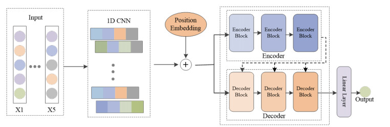
Understanding the patterns of financial activities and predicting their evolution and changes has always been a significant challenge in the field of behavioral finance. Stock price prediction is particularly difficult due to the inherent complexity and stochastic nature of the stock market. Deep learning models offer a more robust solution to nonlinear problems compared to traditional algorithms. In this paper, we propose a simple yet effective fusion model that leverages the strengths of both transformers and convolutional neural networks (CNNs). The CNN component is employed to extract local features, while the Transformer component captures temporal dependencies. To validate the effectiveness of the proposed approach, we conducted experiments on four stocks representing different sectors, including finance, technology, industry, and agriculture. We performed both single-step and multi-step predictions. The experimental results demonstrate that our method significantly improves prediction accuracy, reducing error rates by 45%, 32%, and 36.8% compared to long short-term memory(LSTM), attention-based LSTM, and transformer models.
Citation: Ying Li, Xiangrong Wang, Yanhui Guo. CNN-Trans-SPP: A small Transformer with CNN for stock price prediction[J]. Electronic Research Archive, 2024, 32(12): 6717-6732. doi: 10.3934/era.2024314
Understanding the patterns of financial activities and predicting their evolution and changes has always been a significant challenge in the field of behavioral finance. Stock price prediction is particularly difficult due to the inherent complexity and stochastic nature of the stock market. Deep learning models offer a more robust solution to nonlinear problems compared to traditional algorithms. In this paper, we propose a simple yet effective fusion model that leverages the strengths of both transformers and convolutional neural networks (CNNs). The CNN component is employed to extract local features, while the Transformer component captures temporal dependencies. To validate the effectiveness of the proposed approach, we conducted experiments on four stocks representing different sectors, including finance, technology, industry, and agriculture. We performed both single-step and multi-step predictions. The experimental results demonstrate that our method significantly improves prediction accuracy, reducing error rates by 45%, 32%, and 36.8% compared to long short-term memory(LSTM), attention-based LSTM, and transformer models.

| [1] |
L. Zhang, F. Wang, B. Xu, W. Chi, Q. Wang, T. Sun, Prediction of stock prices based on LM-BP neural network and the estimation of overfitting point by RDCI, Neural Comput. Appl., 30 (2018), 1425–1444. https://doi.org/10.1007/s00521-017-3296-x doi: 10.1007/s00521-017-3296-x

|
| [2] |
Y. LeCun, Y. Bengio, G. Hinton, Deep learning, Nature, 521 (2015), 436–444. https://doi.org/10.1038/nature14539 doi: 10.1038/nature14539
|
| [3] |
R. F. Engle, Autoregressive conditional heteroscedasticity with estimates of the variance of United Kingdom inflation, Econometrica, 50 (1982), 987–1007. https://doi.org/10.2307/1912773 doi: 10.2307/1912773
|
| [4] |
T. Bollerslev, Generalized autoregressive conditional heteroskedasticity, J. Econom., 31 (1986), 307–327. https://doi.org/10.1016/0304-4076(86)90063-1 doi: 10.1016/0304-4076(86)90063-1
|
| [5] |
A. K. Jain, J. Mao, K. M. Mohiuddin, Artificial neural networks: A tutorial, IEEE Comput., 29 (1996), 31–44. https://doi.org/10.1109/2.485891 doi: 10.1109/2.485891
|
| [6] |
J. A. K. Suykens, J. Vandewalle, Least squares support vector machine classifiers, Neural Process. Lett., 9 (1999), 293–300. https://doi.org/10.1023/A:1018628609742 doi: 10.1023/A:1018628609742
|
| [7] |
F. E. H. Tay, L. Cao, Application of support vector machines in financial time series forecasting, IEEE Comput., 29 (2001), 309–317. https://doi.org/10.1016/S0305-0483(01)00026-3 doi: 10.1016/S0305-0483(01)00026-3
|
| [8] | B. Egeli, M. Ozturan, B. Badur, Stock market prediction using artificial neural networks, Decis. Support Syst., 22 (2003), 171–185. |
| [9] |
Y. Kara, M. A. Boyacioglu, Ö. K. Baykan, Predicting direction of stock price index movement using artificial neural networks and support vector machines: The sample of the Istanbul Stock Exchange, Expert Syst. Appl., 38 (2011), 5311–5319. https://doi.org/10.1016/j.eswa.2010.10.027 doi: 10.1016/j.eswa.2010.10.027
|
| [10] |
G. Armano, M. Marchesi, A. Murru, A hybrid genetic-neural architecture for stock indexes forecasting, Inf. Sci., 170 (2005), 3–33. https://doi.org/10.1016/j.ins.2003.03.023 doi: 10.1016/j.ins.2003.03.023
|
| [11] | J. Fu, K. S. Lum, M. N. Nguyen, J. Shi, Stock prediction using fcmac-byy, in Advances in Neural Networks – ISNN 2007, Springer Berlin Heidelberg, 4492 (2007), 346–351. https://doi.org/10.1007/978-3-540-72393-6_42 |
| [12] | R. Choudhry, K. Garg, A hybrid machine learning system for stock market forecasting, Int. J. Comput. Inf. Eng., 2 (2008), 689–692. |
| [13] |
M. Vijh, D. Chandola, V. A. Tikkiwal, A. Kumar, Stock closing price prediction using machine learning techniques, Procedia Comput. Sci., 167 (2020), 599–606. https://doi.org/10.1016/j.procs.2020.03.326 doi: 10.1016/j.procs.2020.03.326
|
| [14] |
K. S. Chandar, H. Punjabi, Cat swarm optimization algorithm tuned multilayer perceptron for stock price prediction, Int. J. Web-Based Learn. Teach. Technol., 17 (2022), 1–15. https://doi.org/10.4018/IJWLTT.303113 doi: 10.4018/IJWLTT.303113
|
| [15] |
Y. Guo, S. Han, C. Shen, Y. Li, X. Yin, Y. Bai, An adaptive SVR for high-frequency stock price forecasting, IEEE Access, 6 (2018), 11397–11404. https://doi.org/10.1109/ACCESS.2018.2806180 doi: 10.1109/ACCESS.2018.2806180
|
| [16] | B. W. Wanjawa, L. Muchemi, ANN model to predict stock prices at stock exchange markets, preprint, arXiv: 1502.06434. |
| [17] | A. Tsantekidis, N. Passalis, A. Tefas, J. Kanniainen, M. Gabbouj, A. Iosifidis, Forecasting stock prices from the limit order book using convolutional neural networks, in 2017 IEEE 19th Conference on Business Informatics (CBI), IEEE, (2017), 7–12. https://doi.org/10.1109/CBI.2017.23 |
| [18] | M. U. Gudelek, S. A. Boluk, A. M. Ozbayoglu, A deep learning based stock trading model with 2-D CNN trend detection, in 2017 IEEE Symposium Series on Computational Intelligence (SSCI), IEEE, (2017), 1–8. https://doi.org/10.1109/SSCI.2017.8285188 |
| [19] | A. J. P. Samarawickrama, T. G. I. Fernando, A recurrent neural network approach in predicting daily stock prices an application to the Sri Lankan stock market, in the 2017 IEEE International Conference on Industrial and Information Systems (ICIIS), IEEE, (2017), 1–6. https://doi.org/10.1109/ICIINFS.2017.8300345 |
| [20] |
M. Roondiwala, H. Patel, S. Varma, Predicting stock prices using LSTM, Int. J. Sci. Res., 6 (2017), 1754–1756. https://doi.org/10.21275/ART20172755 doi: 10.21275/ART20172755
|
| [21] | S. Selvin, R. Vinayakumar, E. A. Gopalakrishnan, V. K. Menon, K. P. Soman, Stock price prediction using LSTM, RNN and CNN-sliding window model, in 2017 International Conference on Advances in Computing, Communications and Informatics (ICACCI), IEEE, (2017), 1643–1647. https://doi.org/10.1109/ICACCI.2017.8126078 |
| [22] |
W. Lu, J. Li, Y. Li, A. Sun, J. Wang, A CNN-LSTM-based model to forecast stock prices, Complexity, 1 (2020), 1–10. https://doi.org/10.1155/2020/6622927 doi: 10.1155/2020/6622927
|
| [23] | A. Vaswani, N. Shazeer, N. Parmar, J. Uszkoreit, L. Jones, A. N. Gomez, et al., Attention is all you need, in Advances in Neural Information Processing Systems, 30 (2017). |
| [24] | Y. Wang, R. Huang, S. Song, Z. Huang, G. Huang, Not all images are worth 16 $\times$ 16 words: dynamic transformers for efficient image recognition, in Advances in Neural Information Processing Systems, 34 (2021), 11960–11973. |
| [25] |
P. Xu, X. Zhu, D. A. Clifton, Multimodal learning with transformers: A survey, IEEE Trans. Pattern Anal. Mach. Intell., 45 (2023), 12113–12132. https://doi.org/10.1109/TPAMI.2023.3275156 doi: 10.1109/TPAMI.2023.3275156
|
| [26] |
S. Lai, Mi. Wang, S. Zhao, G. R. Arce, Predicting high-frequency stock movement with differential Transformer neural network, Electronics, 12 (2023), 2943. https://doi.org/10.3390/electronics12132943 doi: 10.3390/electronics12132943
|
| [27] |
Z. Tao, W. Wu, J. Wang, Series decomposition Transformer with period-correlation for stock market index prediction, Expert Syst. Appl., 237 (2024), 121424. https://doi.org/10.1016/j.eswa.2023.121424 doi: 10.1016/j.eswa.2023.121424
|
| [28] |
A. K. Mishra, J. Renganathan, A. Gupta, Volatility forecasting and assessing risk of financial markets using multi-transformer neural network based architecture, Eng. Appl. Artif. Intell., 133 (2024), 108223. https://doi.org/10.1016/j.engappai.2024.108223 doi: 10.1016/j.engappai.2024.108223
|
| [29] | Z. Shi, MambaStock: Selective state space model for stock prediction, preprint, arXiv: 2402.18959. |
| [30] |
X. Wen, W. Li, Time series prediction based on LSTM-attention-LSTM model, IEEE Access, 11 (2023), 48322–48331. https://doi.org/10.1109/ACCESS.2023.3276628 doi: 10.1109/ACCESS.2023.3276628
|
| [31] |
D. O. Oyewola, S. A. Akinwunmi, T. O. Omotehinwa, Deep LSTM and LSTM-Attention Q-learning based reinforcement learning in oil and gas sector prediction, Knowledge-Based Syst., 284 (2024), 111290. https://doi.org/10.1016/j.knosys.2023.111290 doi: 10.1016/j.knosys.2023.111290
|


Figures(8) / Tables(3)
Ying Li, Xiangrong Wang, Yanhui Guo. CNN-Trans-SPP: A small Transformer with CNN for stock price prediction[J]. Electronic Research Archive, 2024, 32(12): 6717-6732. doi: 10.3934/era.2024314


 DownLoad: