Modeling the role of fish population in mitigating algal bloom

Mohammad Sajid; Arvind Kumar Misra; Ahmed S. Almohaimeed; Mohammad Sajid; Arvind Kumar Misra; Ahmed S. Almohaimeed

doi:10.3934/era.2024269

Electronic Research Archive

2024, Volume 32, Issue 10: 5819-5845. doi: 10.3934/era.2024269

Previous Article Next Article

Research article Special Issues

Modeling the role of fish population in mitigating algal bloom

1.
Department of Mechanical Engineering, College of Engineering, Qassim University, Saudi Arabia
2.
Department of Mathematics, Institute of Science, Banaras Hindu University, Varanasi–221 005, India
3.
Department of Mathematics, College of Science, Qassim University, Saudi Arabia

Received: 18 May 2024 Revised: 04 October 2024 Accepted: 18 October 2024 Published: 29 October 2024

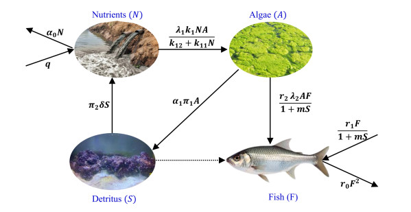
Algal blooms pose a significant threat to the ecological integrity and biodiversity in aquatic ecosystems. In lakes, enriched with nutrients, these blooms result in overgrowth of periphyton, leading to biological clogging, oxygen depletion, and ultimately a decline in ecosystem's health and water quality. In this article, we presented a mathematical model centered around the role of aquatic species (specifically fish population) to alleviate algal blooms. The model analysis revealed significant shifts in dynamics, shedding light on the effectiveness of fish-mediated sustainability strategies to control algal proliferation. Notably, our study identified critical thresholds and regime transitions through the observation of saddle-node bifurcation within the proposed mathematical model. To validate our analytical findings, we have conducted numerical simulations, which provided robust evidence for the resilience of the ecosystem under different scenarios.

Keywords:

Citation: Mohammad Sajid, Arvind Kumar Misra, Ahmed S. Almohaimeed. Modeling the role of fish population in mitigating algal bloom[J]. Electronic Research Archive, 2024, 32(10): 5819-5845. doi: 10.3934/era.2024269

Related Papers:

[1]	Aimin Xu . Some identities involving derangement polynomials and $ r $-Bell polynomials. AIMS Mathematics, 2024, 9(1): 2051-2062. doi: 10.3934/math.2024102
[2]	Feng Qi, Da-Wei Niu, Bai-Ni Guo . Simplifying coefficients in differential equations associated with higher order Bernoulli numbers of the second kind. AIMS Mathematics, 2019, 4(2): 170-175. doi: 10.3934/math.2019.2.170
[3]	Taekyun Kim, Dae San Kim, Hyunseok Lee, Lee-Chae Jang . A note on degenerate derangement polynomials and numbers. AIMS Mathematics, 2021, 6(6): 6469-6481. doi: 10.3934/math.2021380
[4]	Waseem A. Khan, Abdulghani Muhyi, Rifaqat Ali, Khaled Ahmad Hassan Alzobydi, Manoj Singh, Praveen Agarwal . A new family of degenerate poly-Bernoulli polynomials of the second kind with its certain related properties. AIMS Mathematics, 2021, 6(11): 12680-12697. doi: 10.3934/math.2021731
[5]	Hye Kyung Kim . Note on $ r $-central Lah numbers and $ r $-central Lah-Bell numbers. AIMS Mathematics, 2022, 7(2): 2929-2939. doi: 10.3934/math.2022161
[6]	Bai-Ni Guo, Dongkyu Lim, Feng Qi . Series expansions of powers of arcsine, closed forms for special values of Bell polynomials, and series representations of generalized logsine functions. AIMS Mathematics, 2021, 6(7): 7494-7517. doi: 10.3934/math.2021438
[7]	Jongkyum Kwon, Patcharee Wongsason, Yunjae Kim, Dojin Kim . Representations of modified type 2 degenerate poly-Bernoulli polynomials. AIMS Mathematics, 2022, 7(6): 11443-11463. doi: 10.3934/math.2022638
[8]	Rabeb Sidaoui, Abdulghani Muhyi, Khaled Aldwoah, Ayman Alahmade, Mohammed Rabih, Amer Alsulami, Khidir Mohamed . A family of trivariate Gould-Hopper-Bell-Apostol-Type polynomials: Construction and properties. AIMS Mathematics, 2025, 10(6): 13251-13277. doi: 10.3934/math.2025594
[9]	Dojin Kim, Patcharee Wongsason, Jongkyum Kwon . Type 2 degenerate modified poly-Bernoulli polynomials arising from the degenerate poly-exponential functions. AIMS Mathematics, 2022, 7(6): 9716-9730. doi: 10.3934/math.2022541
[10]	Hye Kyung Kim, Dmitry V. Dolgy . Degenerate Catalan-Daehee numbers and polynomials of order $ r $ arising from degenerate umbral calculus. AIMS Mathematics, 2022, 7(3): 3845-3865. doi: 10.3934/math.2022213

Abstract

1. Introduction

Some special polynomials and numbers are diversely used in physics and engineering as well as in mathematics. For example, Bell polynomials play an important role in the studies of water waves which help energy development, mechanical engineering, marine/offshore engineering, hydraulic engineering, etc (see ^{[9,10,11,12,22]}). There are various ways of studying special numbers and polynomials, to mention a few, generating functions, combinatorial methods, $p$ -adic analysis, umbral calculus, differential equations, probability theory, special functions and analytic number theory (see ^[1,2]).

The aim of this paper is to introduce several special polynomials and numbers, and to study their explicit expressions, recurrence relations and identities involving those polynomials and numbers by using generating functions.

Indeed, we introduce Bell polynomials and numbers of the second kind (see (2.3), (2.5)) and poly-Bell polynomials and numbers of the second kind (see (4.1)). The generating function of Bell numbers of the second kind is the compositional inverse of the generating function of Bell numbers minus the constant term. Then Bell polynomials of the second kind are natural extensions of those numbers (see ^[23]). The poly-Bell polynomials of the second kind, which are defined with the help of polylogarithm, become the Bell polynomials of the second kind up to sign when the index of the polylogarithm is $k = 1$ .

We also consider degenerate versions of those numbers and polynomials, namely degenerate Bell numbers and polynomials of the second (see (3.3), (3.5)) and degenerate poly-Bell numbers and polynomials (see (5.1)), and derive similar results. It is worthwhile to note that degenerate versions of many special numbers and polynomials have been explored in recent years with aforementioned tools and many interesting arithmetical and combinatorial results have been obtained (see ^{[14,15,18,19,26]}). In fact, studying degenerate versions can be done not only for polynomials and numbers but also for transcendental functions like gamma functions. For the rest of this section, we recall the necessary facts that are needed throughout this paper.

The Stirling numbers of the first kind, $S_{1}(n, k)$ , are given by

$\begin{equation} \frac{1}{k!}\big(\log(1+t)\big)^{k} = \sum\limits_{n = k}^{\infty}S_{1}(n, k)\frac{t^{n}}{n!}, \quad (k\ge 0), \quad (\mathrm{see}\ [7, 25]), \end{equation}$

(1.1)

As the inversion formula of (1.1), the Stirling numbers of the second kind, $S_{2}(n, k),$ are given by

$\begin{equation} \frac{1}{k!}\big(e^{t}-1\big)^{k} = \sum\limits_{n = k}^{\infty}S_{2}(n, k)\frac{t^{n}}{n!}, \quad (k\ge 0), \quad (\mathrm{see}\ [3, 13-20]). \end{equation}$

(1.2)

It is well known that the Bell polynomials are defined as

$\begin{equation} \mathrm{Bel}_{n}(x) = \sum\limits_{k = 0}^{n}S_{2}(n, k)x^{k}, \quad (n\ge 0), \quad (\mathrm{see}\ [24, 25]). \end{equation}$

(1.3)

From (1.3), we note that

$\begin{equation} e^{x(e^{t}-1)} = \sum\limits_{n = 0}^{\infty}\mathrm{Bel}_{n}(x)\frac{t^{n}}{n!}, \quad (\mathrm{see}\ [4, 7, 8, 17, 27]). \end{equation}$

(1.4)

When $x = 1$ , $\mathrm{Bel}_{n} = \mathrm{Bel}_{n}(1), \ (n\ge 0)$ are called the Bell numbers.

For any $\lambda\in\mathbb{R}$ , the degenerate exponential function is given by

$\begin{equation} e_{\lambda}^{x}(t) = \sum\limits_{n = 0}^{\infty}\frac{(x)_{n, \lambda}}{n!}t^{n} , \quad (\mathrm{see}\ [5, 6, 7, 26, 27]), \end{equation}$

(1.5)

where $(x)_{0, \lambda} = 1, \ (x)_{n, \lambda} = x(x-\lambda)\cdots(x-(n-1)\lambda), \ (n\ge 1)$ .

When $x = 1$ , we write $e_{\lambda}(t) = e_{\lambda}^{1}(t)$ .

The degenerate Stirling numbers of the first kind are defined by

$\begin{equation} \frac{1}{k!}\big(\log_{\lambda}(1+t)\big)^{k} = \sum\limits_{n = k}^{\infty}S_{1, \lambda}(n, k)\frac{t^{n}}{n!}, \ (k\ge 0), \ (\mathrm{see}\ [15]), \end{equation}$

(1.6)

where

$\begin{equation} \log_{\lambda}(1+t) = \sum\limits_{n = 1}^{\infty}\lambda^{n-1}(1)_{n, 1/\lambda}\frac{t^{n}}{n!}, \quad (\mathrm{see}\ [15]). \end{equation}$

(1.7)

In view of (1.2), the degenerate Stirling numbers of the second kind are defined by

$\begin{equation} \frac{1}{k!}\big(e_{\lambda}(t)-1\big)^{k} = \sum\limits_{n = k}^{\infty}S_{2}(n, k)\frac{t^{n}}{n!}, \quad (\mathrm{see}\ [15]). \end{equation}$

(1.8)

In ^[17], the degenerate Bell polynomials are defined by

$\begin{equation} e_{\lambda}^{x}\big(e_{\lambda}(t)-1\big) = \sum\limits_{n = 0}^{\infty}\mathrm{Bel}_{n, \lambda}(x)\frac{t^{n}}{n!}. \end{equation}$

(1.9)

When $x = 1$ , $\mathrm{Bel}_{n, \lambda} = \mathrm{Bel}_{n, \lambda}(1), \ (n\ge 0)$ , are called the Bell numbers.

From (1.8) and (1.9), we note that

$\begin{equation} \mathrm{Bel}_{n, \lambda}(x) = \sum\limits_{k = 0}^{n}S_{2, \lambda}(n, k)(x)_{k, \lambda}, \ (n\ge 0), \ (\mathrm{see}\ [17]). \end{equation}$

(1.10)

The polylogarithm of index $k$ is given by

$\begin{equation} \mathrm{Li}_{k}(x) = \sum\limits_{n = 1}^{\infty}\frac{x^{n}}{n^{k}}, \quad (k\in\mathbb{Z}, \ |x| < 1), \quad(\mathrm{see}\ [3, 13, 14, 16, 21]). \end{equation}$

(1.11)

Note that $\mathrm{Li}_{1}(x) = -\log(1-x)$ .

Recently, the degenerate polylogarithm is defined as

$\begin{equation} \mathrm{Li}_{k, \lambda}(x) = \sum\limits_{n = 1}^{\infty}\frac{(-\lambda)^{n-1}(1)_{n, 1/\lambda}}{(n-1)!n^{k}}x^{n}, \quad(|x| < 1, \ k\in\mathbb{Z}), \quad(\mathrm{see}\ [15]). \end{equation}$

(1.12)

Note that $\mathrm{Li}_{1, \lambda}(x) = -\log_{\lambda}(1-x)$ .

Here we mention that, to our best knowledge, the results of this paper are new.

2. Bell polynomials of the second kind

From (1.4), we note that

$e^{x(e^{t}-1)} = \sum\limits_{n = 0}^{\infty}\mathrm{Bel}_{n}(x)\frac{t^{n}}{n!}$

Let $x = 1$ . Then we have

$\begin{equation} e^{e^{t}-1}-1 = \sum\limits_{n = 1}^{\infty}\mathrm{Bel}_{n}\frac{t^{n}}{n!}. \end{equation}$

(2.1)

Let $f(t) = e^{e^{t}-1}-1$ . Then the compositional inverse of $f(t)$ is given by

$\begin{equation} f^{-1}(t) = \log\big(1+\log(1+t)\big). \end{equation}$

(2.2)

We consider the new type Bell numbers, called Bell numbers of the second kind, defined by

$\begin{equation} \log\big(1+\log(1+t)\big) = \sum\limits_{n = 1}^{\infty}\mathrm{bel}_{n}\frac{t^{n}}{n!}. \end{equation}$

(2.3)

Now, we observe that

$\begin{align} &\log\big(1+\log(1+t)\big) = \sum\limits_{k = 1}^{\infty}\frac{(-1)^{k-1}}{k}\big(\log(1+t)\big)^{k} \\ & = \sum\limits_{k = 1}^{\infty}(-1)^{k-1}(k-1)!\frac{1}{k!}\big(\log(1+t)\big)^{k} = \sum\limits_{k = 1}^{\infty}(-1)^{k-1}(k-1)!\sum\limits_{n = k}^{\infty}S_{1}(n, k)\frac{t^{n}}{n!} \\ & = \sum\limits_{n = 1}^{\infty}\bigg(\sum\limits_{k = 1}^{n}(-1)^{k-1}(k-1)!S_{1}(n, k) \bigg)\frac{t^{n}}{n!}. \end{align}$

(2.4)

Therefore, by (2.3) and (2.4), we obtain the following theorem.

Theorem 1. For $n\ge 1$ , we have

$(-1)^{n-1}\mathrm{bel}_{n} = \sum\limits_{k = 1}^{n}(k-1)!{n \brack k},$

where ${n \brack k}$ are the unsigned Stirling numbers of the first kind.

Also, we consider the new type Bell polynomials, called Bell polynomials of the second kind, defined by

$\begin{equation} \mathrm{bel}_{n}(x) = \sum\limits_{k = 1}^{n}(-1)^{k-1}(k-1)!S_{1}(n, k)x^{k}, \quad (n\ge 1). \end{equation}$

(2.5)

From (2.5), we can derive the following equation.

$\begin{align} \sum\limits_{n = 1}^{\infty} \mathrm{bel}_{n}(x)\frac{t^{n}}{n!}& = \sum\limits_{n = 1}^{\infty}\bigg(\sum\limits_{k = 1}^{n}(-1)^{k-1}(k-1)!S_{1}(n, k)x^{k}\bigg)\frac{t^{n}}{n!} \\ & = \sum\limits_{k = 1}^{\infty}(-1)^{k-1}(k-1)!x^{k}\sum\limits_{n = k}^{\infty}S_{1}(n, k)\frac{t^{n}}{n!} \\ & = \sum\limits_{k = 1}^{\infty}\frac{(-1)^{k-1}k!}{k}x^{k}\frac{1}{k!}\big(\log(1+t)\big)^{k} \\ & = \sum\limits_{k = 1}^{\infty}\frac{(-1)^{k-1}}{k}x^{k}\big(\log(1+t)\big)^{k} = \log (1+x\log(1+t)). \end{align}$

(2.6)

Thus the generating function of Bell polynomials of the second kind is given by

$\begin{equation} \log\big(1+x\log(1+t)\big) = \sum\limits_{n = 1}^{\infty}\mathrm{bel}_{n}(x)\frac{t^{n}}{n!}. \end{equation}$

(2.7)

Note here that $\mathrm{bel}_{n} = \mathrm{bel}_{n}(1)$ . From (2.7), we note that

$\begin{equation} \frac{x}{\big(1+x\log(1+t)\big)(1+t)} = \frac{d}{dt}\log\big(1+x\log(1+t)\big) = \sum\limits_{n = 0}^{\infty}\mathrm{bel}_{n+1}(x)\frac{t^{n}}{n!} . \end{equation}$

(2.8)

Replacing $t$ by $e^{t}-1$ in (2.8), we get

$\begin{align} \frac{x}{1+xt}e^{-t}\ & = \ \sum\limits_{k = 0}^{\infty}\mathrm{bel}_{k+1}(x)\frac{1}{k!}\big(e^{t}-1\big)^{k} \\ & = \ \sum\limits_{k = 0}^{\infty}\mathrm{bel}_{k+1}(x)\sum\limits_{n = k} ^{\infty}S_{2}(n, k)\frac{t^{n}}{n!} \\ & = \ \sum\limits_{n = 0}^{\infty}\bigg(\sum\limits_{k = 0}^{n}\mathrm{bel}_{k+1}(x)S_{2}(n, k)\bigg)\frac{t^{n}}{n!}. \end{align}$

(2.9)

Taking $x = -1$ in (2.9), we have

$\begin{equation} \sum\limits_{n = 0}^{\infty}\bigg(\sum\limits_{k = 0}^{n}\mathrm{bel}_{k+1}(-1)S_{2}(n, k)\bigg)\frac{t^{n}}{n!} = -\frac{1}{1-t}e^{-t} = -\sum\limits_{n = 0}^{\infty}d_{n}\frac{t^{n}}{n!}, \end{equation}$

(2.10)

where $d_{n}$ is the derangement number (see ^[19]).

Therefore, by comparing the coefficients on both sides of (2.10), we obtain the following theorem.

Theorem 2. For $n\ge 0$ , we have

$\sum\limits_{k = 0}^{n}\mathrm{bel}_{k+1}(-1)S_{2}(n, k) = -d_{n}.$

Replacing $t$ by $e^{e^{t}-1}-1$ in (2.3), we get

$\begin{align} t& = \sum\limits_{k = 1}^{\infty}\mathrm{bel}_{k}\frac{1}{k!}\Big(e^{e^{t}-1}-1\Big)^{k} = \sum\limits_{k = 1}^{\infty}\mathrm{bel}_{k}\sum\limits_{j = k}^{\infty}S_{2}(j, k)\frac{1}{j!} \big(e^{t}-1\big)^{j} \\ & = \sum\limits_{j = 1}^{\infty}\sum\limits_{k = 1}^{j}\mathrm{bel}_{k}S_{2}(j, k)\sum\limits_{n = j}^{\infty}S_{2}(n, k)\frac{t^{n}}{n!} \\ & = \sum\limits_{n = 1}^{\infty}\bigg(\sum\limits_{j = 1}^{n}\sum\limits_{k = 1}^{j}\mathrm{bel}_{k}S_{2}(j, k)S_{2}(n, j)\bigg)\frac{t^{n}}{n!}. \end{align}$

(2.11)

Thus we obtain following theorem.

Theorem 3. For $n\ge 2$ , we have

$\sum\limits_{j = 1}^{n}\sum\limits_{k = 1}^{j}\mathrm{bel}_{k}S_{2}(j, k)S_{2}(n, j) = 0, \, \, \, \mathrm{and}\, \, \, \mathrm{bel}_{1} = 1.$

Replacing $t$ by $e^{t}-1$ in (2.7), we get

$\begin{align} \log(1+xt)\ & = \ \sum\limits_{k = 1}^{\infty}\mathrm{bel}_{k}(x)\frac{1}{k!}\big(e^{t}-1\big)^{k} \\ & = \ \sum\limits_{k = 1}^{\infty}\mathrm{bel}_{k}(x)\sum\limits_{n = k}^{\infty}S_{2}(n, k)\frac{t^{n}}{n!} \\ & = \ \sum\limits_{n = 1}^{\infty}\bigg(\sum\limits_{k = 1}^{n}\mathrm{bel}_{k}(x)S_{2}(n, k)\bigg)\frac{t^{n}}{n!}. \end{align}$

(2.12)

On the other hand,

$\begin{equation} \log(1+xt) = \sum\limits_{n = 1}^{\infty}\frac{(-1)^{n-1}}{n}x^{n}t^{n}. \end{equation}$

(2.13)

Therefore, by (2.12) and (2.13), we obtain the following theorem.

Theorem 4. For $n\ge 1$ , we have

$x^{n} = \frac{(-1)^{n-1}}{(n-1)!}\sum\limits_{k = 1}^{n}\mathrm{bel}_{k}(x)S_{2}(n, k).$

In particular,

$1 = \frac{(-1)^{n-1}}{(n-1)!}\sum\limits_{k = 1}^{n}\mathrm{bel}_{k}S_{2}(n, k).$

3. Degenerate Bell polynomials of the second kind

From (1.3), we note that

$\begin{equation} e_{\lambda}\big(e_{\lambda}(t)-1\big)-1 = \sum\limits_{n = 1}^{\infty}\mathrm{Bel}_{n, \lambda}\frac{t^{n}}{n!}. \end{equation}$

(3.1)

Let $f_{\lambda}(t) = e_{\lambda}\big(e_{\lambda}(t)-1\big)-1$ . Then the compositional inverse of $f_{\lambda}(t)$ is given by

$\begin{equation} f_{\lambda}^{-1}(t) = \log_{\lambda}\big(1+\log_{\lambda}(1+t)\big). \end{equation}$

(3.2)

We consider the new type degenerate Bell numbers, called degenerate Bell numbers of the second kind, defined by

$\begin{equation} \log_{\lambda}\big(1+\log_{\lambda}(1+t)\big) = \sum\limits_{n = 1}^{\infty}\mathrm{bel}_{n, \lambda}\frac{t^{n}}{n!}. \end{equation}$

(3.3)

Now, we observe that

$\begin{align} \log_{\lambda}\big(1+\log_{\lambda}(1+t)\big)\ & = \ \sum\limits_{k = 1}^{\infty}\lambda^{k-1}(1)_{k, 1/\lambda}\frac{1}{k!}\big(\log_{\lambda}(1+t)\big)^{k} \\ & = \ \sum\limits_{k = 1}^{\infty}\lambda^{k-1}(1)_{k, 1/\lambda}\sum\limits_{n = k}^{\infty}S_{1, \lambda}(n, k)\frac{t^{n}}{n!}. \\ & = \ \sum\limits_{n = 1}^{\infty}\bigg(\sum\limits_{k = 1}^{n}\lambda^{k-1}(1)_{k, 1/\lambda}S_{1, \lambda}(n, k)\bigg)\frac{t^{n}}{n!}. \end{align}$

(3.4)

Therefore, by (3.3) and (3.4), we obtain the following theorem.

Theorem 5. For $n\ge 1$ , we have

$\mathrm{bel}_{n, \lambda} = \sum\limits_{k = 1}^{n}\lambda^{k-1}(1)_{k, 1/\lambda}S_{1, \lambda}(n, k).$

Also, we define the degenerate Bell polynomials of second kind by

$\begin{equation} \mathrm{bel}_{n, \lambda}(x) = \sum\limits_{k = 1}^{n}\lambda^{k-1}(1)_{k, 1/\lambda}S_{1, \lambda}(n, k)x^{k}. \end{equation}$

(3.5)

Note that $\mathrm{bel}_{n, \lambda} = \mathrm{bel}_{n, \lambda}(1)$ .

From (3.5), we note that

$\begin{align} \sum\limits_{n = 1}^{\infty}\mathrm{bel}_{n, \lambda}(x)\frac{t^{n}}{n!}\ & = \ \sum\limits_{n = 1}^{\infty}\bigg(\sum\limits_{k = 1}^{n}\lambda^{k-1}(1)_{k, 1/\lambda}S_{1, \lambda}(n, k)x^{k}\bigg)\frac{t^{n}}{n!} \\ & = \ \sum\limits_{k = 1}^{\infty}\lambda^{k-1}(1)_{k, 1/\lambda}x^{k}\sum\limits_{n = k}^{\infty}S_{1, \lambda}(n, k)\frac{t^{n}}{n!} \\ & = \ \sum\limits_{k = 1}^{\infty}\lambda^{k-1}(1)_{k, 1/\lambda}x^{k}\frac{1}{k!}\big(\log_{\lambda}(1+t)\big)^{k} \\ & = \ \log_{\lambda}\big(1+x\log_{\lambda}(1+t)\big). \end{align}$

(3.6)

Thus the generating function of $\mathrm{bel}_{n, \lambda}(x)$ is given by

$\begin{equation} \log_{\lambda}\big(1+x\log_{\lambda}(1+t)\big) = \sum\limits_{n = 1}^{\infty}\mathrm{bel}_{n, \lambda}(x)\frac{t^{n}}{n!}. \end{equation}$

(3.7)

Replacing $t$ by $e_{\lambda}(t)-1$ in (3.7), we get

$\begin{align} \log_{\lambda}(1+xt)\ & = \ \sum\limits_{k = 1}^{\infty}\mathrm{bel}_{k, \lambda}(x)\frac{1}{k!}\big(e_{\lambda}(t)-1\big)^{k} \\ & = \ \sum\limits_{k = 1}^{\infty}\mathrm{bel}_{k, \lambda}(x)\sum\limits_{n = k}^{\infty}S_{2, \lambda}(n, k)\frac{t^{n}}{n!} \\ & = \ \sum\limits_{n = 1}^{\infty}\bigg(\sum\limits_{k = 1}^{n}\mathrm{bel}_{k, \lambda}(x)S_{2, \lambda}(n, k)\bigg)\frac{t^{n}}{n!}. \end{align}$

(3.8)

On the other hand,

$\begin{equation} \log_{\lambda}(1+xt) = \sum\limits_{n = 1}^{\infty}\lambda^{n-1}(1)_{n, 1/\lambda}x^{n}\frac{t^{n}}{n!}. \end{equation}$

(3.9)

Therefore, by (3.8) and (3.9), we obtain the following theorem.

Theorem 6. For $n\ge 1$ , we have

$x^{n} = \frac{\lambda^{1-n}}{(1)_{n, 1/\lambda}}\sum\limits_{k = 1}^{n}\mathrm{bel}_{k, \lambda}(x)S_{2, \lambda}(n, k).$

In particular,

$\lambda^{n-1}(1)_{n, 1/\lambda} = \sum\limits_{k = 1}^{n}\mathrm{bel}_{k, \lambda}S_{2, \lambda}(n, k).$

Replacing $t$ by $e_{\lambda}\big(e_{\lambda}(t)-1\big)-1$ in (3.3), we have

$\begin{align} t\ & = \sum\limits_{k = 1}^{\infty}\mathrm{bel}_{k, \lambda}\frac{1}{k!} \big(e_{\lambda}(e_{\lambda}(t)-1)-1\big)^{k} \\ & = \sum\limits_{k = 1}^{\infty}\mathrm{bel}_{k, \lambda}\sum\limits_{j = k}^{\infty}S_{2, \lambda}(j, k)\frac{1}{j!}\big(e_{\lambda}(t)-1\big)^{j} \\ & = \ \sum\limits_{j = 1}^{\infty}\bigg(\sum\limits_{k = 1}^{j}\mathrm{bel}_{k, \lambda}S_{2, \lambda}(j, k)\bigg)\sum\limits_{n = j}^{\infty}S_{2, \lambda}(n, j)\frac{t^{n}}{n!} \\ & = \ \sum\limits_{n = 1}^{\infty}\bigg(\sum\limits_{j = 1}^{n}\sum\limits_{k = 1}^{j}\mathrm{bel}_{k, \lambda}S_{2, \lambda}(j, k)S_{2, \lambda}(n, j)\bigg)\frac{t^{n}}{n!}. \end{align}$

(3.10)

Therefore, by comparing the coefficients on both sides of (3.10), we obtain the following theorem.

Theorem 7. For $n\ge 2$ , we have

$\sum\limits_{j = 1}^{n}\sum\limits_{k = 1}^{j}\mathrm{bel}_{k, \lambda}S_{2, \lambda}(j, k)S_{2, \lambda}(n, j) = 0, \, \, \, \mathrm{and}\, \, \, \mathrm{bel}_{1, \lambda} = 1.$

4. Poly-Bell polynomials of the second kind

Now, we consider the poly-Bell polynomials of the second kind which are defined as

$\begin{equation} \mathrm{Li}_{k}\big(-x\log(1-t)\big) = \sum\limits_{n = 1}^{\infty}\mathrm{bel}_{n}^{(k)}(x)\frac{t^{n}}{n!}. \end{equation}$

(4.1)

When $x = 1$ , $\mathrm{bel}_{n}^{(k)} = \mathrm{bel}_{n}^{(k)}(1)$ are called the poly-Bell numbers of the second kind.

From (1.11), we note that

$\begin{align} \mathrm{Li}_{k}\big(-x\log(1-t)\big)\ & = \ \sum\limits_{l = 1}^{\infty}\frac{(-1)^{l}}{l^{k}}x^{l}l!\frac{1}{l!}\big(\log(1-t)\big)^{l} \\ & = \ \sum\limits_{l = 1}^{\infty}\frac{(-1)^{l}}{l^{k-1}}(l-1)!x^{l}\sum\limits_{n = l}^{\infty}(-1)^{n}S_{1}(n, l)\frac{t^{n}}{n!} \\ & = \ \sum\limits_{n = 1}^{\infty}\bigg(\sum\limits_{l = 1}^{n}\frac{(-1)^{n-l}}{l^{k-1}}(l-1)!x^{l}S_{1}(n, l)\bigg)\frac{t^{n}}{n!}. \end{align}$

(4.2)

Therefore, by (4.1) and (4.2), we obtain the following theorem.

Theorem 8. For $n\ge 1$ , we have

$\mathrm{bel}_{n}^{(k)}(x) = \sum\limits_{l = 1}^{n}\frac{x^{l}}{l^{k-1}}(l-1)!{n \brack l}.$

In particular,

$\mathrm{bel}_{n}^{(k)} = \sum\limits_{l = 1}^{n}\frac{1}{l^{k-1}}(l-1)!{n \brack l}.$

Note that

$\mathrm{bel}_{n}^{(1)}(x) = \sum\limits_{l = 1}^{n}x^{l}(l-1)! {n \brack l} = (-1)^{n-1}\mathrm{bel}_{n}(x).$

Indeed,

$\begin{align*} \mathrm{Li}_{1}\big(-x\log(1-t)\big)\ & = \ -\log\big(1+x\log(1-t)\big) \\ & = \ \sum\limits_{n = 1}^{\infty}\mathrm{bel}_{n}(x)(-1)^{n-1}\frac{t^{n}}{n!}. \end{align*}$

Replacing $t$ by $1-e^{-t}$ in (4.1), we get

$\begin{align} \mathrm{Li}_{k}(xt)\ & = \ \sum\limits_{l = 1}^{\infty}\mathrm{bel}_{l}^{(k)}(x)\frac{1}{l!}\big(1-e^{-t}\big)^{l} \\ & = \ \sum\limits_{l = 1}^{\infty}\mathrm{bel}_{l}^{(k)}(x)(-1)^{l}\sum\limits_{n = l}^{\infty}S_{2}(n, l)(-1)^{n}\frac{t^{n}}{n!}. \\ & = \ \sum\limits_{n = 1}^{\infty}\bigg(\sum\limits_{l = 1}^{n}(-1)^{n-l}\mathrm{bel}_{l}^{(k)}(x)S_{2}(n, l)\bigg)\frac{t^{n}}{n!}. \end{align}$

(4.3)

From (1.11) and (4.3), we note that

$\begin{equation} \frac{x^{n}}{n^{k}} = \frac{1}{n!}\sum\limits_{l = 1}^{n}(-1)^{n-l}\mathrm{bel}_{l}^{(k)}(x)S_{2}(n, l). \end{equation}$

(4.4)

Therefore, by (4.4), we obtain the following theorem.

Theorem 9. For $n\ge 1$ , we have

$x^{n} = \frac{n^{k-1}}{(n-1)!}\sum\limits_{l = 1}^{n}(-1)^{n-l}\mathrm{bel}_{l}^{(k)}(x)S_{2}(n, l).$

5. Degenerate poly-Bell polynomials of the second kind

We define the degenerate poly-Bell polynomials of the second kind by

$\begin{equation} \mathrm{Li}_{k, \lambda}\big(-x\log_{\lambda}(1-t)\big) = \sum\limits_{n = 1}^{\infty}\mathrm{bel}_{n, \lambda}^{(k)}(x)\frac{t^{n}}{n!}. \end{equation}$

(5.1)

When $x = 1$ , $\mathrm{bel}_{n, \lambda}^{(k)} = \mathrm{bel}_{n, \lambda}^{(k)}(1)$ are called the degenerate poly-Bell numbers of the second.

From (2.1), we note that

$\begin{align} \mathrm{Li}_{k, \lambda}\big(-x\log_{\lambda}(1-t)\ & = \ \sum\limits_{l = 1}^{\infty}\frac{(-\lambda)^{l-1}(1)_{l, 1/\lambda}}{(l-1)!l^{k}}\big(-x\log_{\lambda}(1-t)\big)^{l} \\ & = \ -\sum\limits_{l = 1}^{\infty}\frac{(1)_{l, 1/\lambda}}{l^{k-1}}\lambda^{l-1}x^{l}\frac{1}{l!}\big(\log_{\lambda}(1-t)\big)^{l}. \\ & = -\sum\limits_{l = 1}^{\infty}\frac{(1)_{l, 1/\lambda}}{l^{k-1}}\lambda^{l-1}x^{l}\sum\limits_{n = l}^{\infty}S_{1, \lambda}(n, l)(-1)^{n}\frac{t^{n}}{n!} \\ & = \ \sum\limits_{n = 1}^{\infty}\bigg((-1)^{n-1}\sum\limits_{l = 1}^{n}\frac{1}{l^{k-1}}(1)_{l, 1/\lambda}\lambda^{l-1}x^{l}S_{1, \lambda}(n, l)\bigg)\frac{t^{n}}{n!}. \end{align}$

(5.2)

Therefore, by (5.1) and (5.2), we obtain the following theorem.

Theorem 10. For $n\ge 1$ , we have

$(-1)^{n-1}\mathrm{bel}_{n, \lambda}^{(k)}(x) = \sum\limits_{l = 1}^{n}\frac{1}{l^{k-1}}(1)_{l, 1/\lambda}\lambda^{l-1}x^{l}S_{1, \lambda}(n, l).$

For $k = 1$ , we have

$(-1)^{n-1}\mathrm{bel}_{n, \lambda}^{(1)}(x) = \sum\limits_{l = 1}^{n}(1)_{l, 1/\lambda}\lambda^{l-1}x^{l}S_{1, \lambda}(n, l) = \mathrm{bel}_{n, \lambda}(x), \quad (n\ge 0).$

Indeed,

$\mathrm{Li}_{1, \lambda}\big(-x\log_{\lambda}(1-t)\big) = -\log_{\lambda}\big(1+x\log_{\lambda}(1-t)\big) = \sum\limits_{n = 1}^{\infty}(-1)^{n-1}\mathrm{bel}_{n, \lambda}(x)\frac{t^{n} }{n!}.$

Replacing $t$ by $1-e_{\lambda}(-t)$ in (5.1), we get

$\begin{align} \mathrm{Li}_{k, \lambda}(xt)\ & = \ \sum\limits_{l = 1}^{\infty} \mathrm{bel}_{l, \lambda}^{(k)}(x)\frac{1}{l!}\big(1-e_{\lambda}(-t)\big)^{l} \\ & = \ \sum\limits_{l = 1}^{\infty} \mathrm{bel}_{l, \lambda}^{(k)}(x)(-1)^{l}\frac{1}{l!}\big(e_{\lambda}(-t)-1\big)^{l} \\ & = \ \sum\limits_{l = 1}^{\infty} \mathrm{bel}_{l, \lambda}^{(k)}(x)(-1)^{l}\sum\limits_{n = l}^{\infty}S_{2, \lambda}(n, l)(-1)^{n}\frac{t^{n}}{n!} \\ & = \ \sum\limits_{n = 1}^{\infty}\bigg(\sum\limits_{l = 1}^{n}(-1)^{n-l} \mathrm{bel}_{l, \lambda}^{(k)}(x)S_{2, \lambda}(n, l)\bigg)\frac{t^{n}}{n!}. \end{align}$

(5.3)

On the other hand,

$\begin{equation} \mathrm{Li}_{k, \lambda}(xt) = \sum\limits_{n = 1}^{\infty}\frac{(-\lambda)^{n-1}(1)_{n, 1/\lambda}}{(n-1)!n^{k}}x^{n}t^{n} = \sum\limits_{n = 1}^{\infty}\frac{(-\lambda)^{n-1}(1)_{n, 1/\lambda}}{n^{k-1}}x^{n}\frac{t^{n}}{n!}. \end{equation}$

(5.4)

From (5.3) and (5.4), we get the following result.

Theorem 11. For $n \ge 1$ , we have

$\frac{(-\lambda)^{n-1}(1)_{n, 1/\lambda}}{n^{k-1}}x^{n} = \sum\limits_{l = 1}^{n}(-1)^{n-l}\mathrm{bel}_{l, \lambda}^{(k)}(x)S_{2, \lambda}(n, l).$

6. Conclusions

Many special polynomials and numbers are widely used in physics and engineering as well as in mathematics. In recent years, degenerate versions of some special polynomials and numbers have been studied by means of various different tools. Here we introduced Bell polynomials of the second kind, poly-Bell polynomials of the second kind and their degenerate versions, namely degenerate Bell polynomials of the second kind and degenerate poly-Bell polynomials of the second kind. By using generating functions, we explored their explicit expressions, recurrence relations and some identities involving those polynomials and numbers.

It is one of our future projects to continue this line of research, namely to explore many special numbers and polynomials and their degenerate versions with the help of various different tools.

Acknowledgments

This work was supported by the Basic Science Research Program, the National Research Foundation of Korea, (NRF-2021R1F1A1050151).

Conflict of interest

The authors declare no conflict of interest.

References

[1]	B. Bhagowati K. U. Ahamad, A review on lake eutrophication dynamics and recent developments in lake modeling, Ecohydrol. Hydrobiol., 19 (2019), 155–166. https://doi.org/10.1016/j.ecohyd.2018.03.002 doi: 10.1016/j.ecohyd.2018.03.002
[2]	H. Wang, H. Wang, Mitigation of lake eutrophication: Loosen nitrogen control and focus on phosphorus abatement, Prog. Nat. Sci., 19 (2009), 1445–1451. https://doi.org/10.1016/j.pnsc.2009.03.009 doi: 10.1016/j.pnsc.2009.03.009
[3]	A. K. Misra, P. Chandra, V. Raghavendra, Modeling the depletion of dissolved oxygen in a lake due to algal bloom: Effect of time delay, Adv. Water Resour., 34 (2011), 1232–1238. https://doi.org/10.1016/j.advwatres.2011.05.010 doi: 10.1016/j.advwatres.2011.05.010
[4]	X. Li, T. Yan, R. Yu, M. Zhou, A review of Karenia mikimotoi: Bloom events, physiology, toxicity and toxic mechanism, Harmful Algae, 90 (2019), 101702. https://doi.org/10.1016/j.hal.2019.101702 doi: 10.1016/j.hal.2019.101702
[5]	M. Pal, P. J. Yesankar, A. Dwivedi, A. Qureshi, Biotic control of harmful algal blooms (HABs): A brief review, J. Environ. Manage., 268 (2020), 110687. https://doi.org/10.1016/j.jenvman.2020.110687 doi: 10.1016/j.jenvman.2020.110687
[6]	L. M. Grattan, S. Holobaugh, J. G. Morris Jr, Harmful algal blooms and public health, Harmful Algae, 57 (2016), 2–8. https://doi.org/10.1016/j.hal.2016.05.003 doi: 10.1016/j.hal.2016.05.003
[7]	S. Xiang, Y. Han, C. Jiang, M. Li, L. Wei, J. Fu, et al., Composite biologically active filter (BAF) with zeolite, granular activated carbon, and suspended biological carrier for treating algae-laden raw water, J. Water Process Eng., 42, (2021), 102188. https://doi.org/10.1016/j.jwpe.2021.102188
[8]	Y. Peng, W. Zhang, X. Yang, Z. Zhang, G. Zhu, S. Zhou, Current status and prospects of algal bloom early warning technologies: A review, J. Environ. Manage., 349 (2024), 119510. https://doi.org/10.1016/j.jenvman.2023.119510 doi: 10.1016/j.jenvman.2023.119510
[9]	Y. Peng, X. Xiao, B. Ren, Z. Zhang, J. Luo, X. Yang, et al., Biological activity and molecular mechanism of inactivation of Microcystis aeruginosa by ultrasound irradiation, J. Hazard. Mater., 468 (2024), 133742. https://doi.org/10.1016/j.jhazmat.2024.133742 doi: 10.1016/j.jhazmat.2024.133742
[10]	C. Chen, X. Pang, Y. Wang, M. Kong, L. Long, M. Xu, et al., Antioxidant responses and microcystins accumulation in Corbicula fluminea following the control of algal blooms using chitosan-modified clays, J. Soils Sediments, 21 (2021), 3505–3514. https://doi.org/10.1007/s11368-021-03022-w doi: 10.1007/s11368-021-03022-w
[11]	K. Liu, L. Jiang, J. Yang, S. Ma, K. Chen, Y. Zhang, et al., Comparison of three flocculants for heavy cyanobacterial bloom mitigation and subsequent environmental impact, J. Oceanol. Limnol., 40 (2022), 1764–1773. https://doi.org/10.1007/s00343-022-1351-7 doi: 10.1007/s00343-022-1351-7
[12]	D. E. Berthold, A. Elazar, F. Lefler, C. Marble, H. D. Laughinghouse IV, Control of algal growth on greenhouse surfaces using commercial algaecides, Sci. Agri., 78 (2020), e20180292. https://doi.org/10.1590/1678-992x-2018-0292 doi: 10.1590/1678-992x-2018-0292
[13]	P. Laue, H. Bahrs, S. Chakrabarti, C. E. Steinberg, Natural xenobiotics to prevent cyanobacterial and algal growth in freshwater: Contrasting efficacy of tannic acid, gallic acid, and gramine, Chemosphere, 104 (2014), 212–220. https://doi.org/10.1016/j.chemosphere.2013.11.029 doi: 10.1016/j.chemosphere.2013.11.029
[14]	R. Sun, P. Sun, J. Zhang, S. Esquivel-Elizondo, Y. Wu, Microorganisms-based methods for harmful algal blooms control: A review, Bioresour. Technol., 248 (2018), 12–20. https://doi.org/10.1016/j.biortech.2017.07.175 doi: 10.1016/j.biortech.2017.07.175
[15]	I. Domaizon, J. Devaux, A new approach in biomanipulation techniques: Use of a phytoplanktivorous fish, the silver carp (Hypophthalmichthys molitrix), Anne Biol., 38 (1999). https://doi.org/10.1016/S0003-5017(99)80028-2
[16]	M. K. Ekvall, P. Urrutia-Cordero, L. A. Hansson, Linking cascading effects of fish predation and zooplankton grazing to reduced cyanobacterial biomass and toxin levels following biomanipulation, PloS One, 9 (2014), 112956. https://doi.org/10.1371/journal.pone.0112956 doi: 10.1371/journal.pone.0112956
[17]	G. W. Waajen, N. C. Van Bruggen, L. M. D. Pires, W. Lengkeek, M. Lürling, Biomanipulation with quagga mussels (Dreissena rostriformis bugensis) to control harmful algal blooms in eutrophic urban ponds, Ecol. Eng., 90 (2016), 141–150. https://doi.org/10.1016/j.ecoleng.2016.01.036 doi: 10.1016/j.ecoleng.2016.01.036
[18]	A. A. Voinov, A. P. Tonkikh, Qualitative model of eutrophication in macrophyte lakes, Ecol. Model., 35, (1987), 211–226. https://doi.org/10.1016/0304-3800(87)90113-X
[19]	M. Scheffer, S. Carpenter, J. A. Foley, C. Folke, B. Walker, Catastrophic shifts in ecosystems, Nature, 413 (2001) 591–596. https://doi.org/10.1038/35098000
[20]	X. Mao, X. Wei, D. Yuan, Y. Jin, X. Jin, An ecological-network-analysis based perspective on the biological control of algal blooms in Ulansuhai Lake, China, Ecol. Model., 386 (2018), 11–19. https://doi.org/10.1016/j.ecolmodel.2018.07.020 doi: 10.1016/j.ecolmodel.2018.07.020
[21]	A. K. Misra, Mathematical modeling and analysis of eutrophication of water bodies caused by nutrients, Nonlinear Anal. Model. Control, 12 (2007), 511–524. https://doi.org/10.15388/NA.2007.12.4.14683 doi: 10.15388/NA.2007.12.4.14683
[22]	P. K. Tiwari, S. Samanta, F. Bona, E. Venturino, A. K. Misra, The time delays influence on the dynamical complexity of algal blooms in the presence of bacteria, Ecol. Complex., 39 (2019), 100769. https://doi.org/10.1016/j.ecocom.2019.100769 doi: 10.1016/j.ecocom.2019.100769
[23]	J. B. Shukla, A. K. Misra, P. Chandra, Mathematical modeling and analysis of the depletion of dissolved oxygen in eutrophied water bodies affected by organic pollutants, Nonlinear Anal. Real World Appl., 9, (2008), 1851–1865. https://doi.org/10.1016/j.nonrwa.2007.05.016
[24]	H. Yan, D. Wu, Y. Huang, G. Wang, M. Shang, J. Xu, et al., Water eutrophication assessment based on rough set and multidimensional cloud model, Chemometr Intell. Lab. Syst., 164 (2017), 103–112. https://doi.org/10.1016/j.chemolab.2017.02.005 doi: 10.1016/j.chemolab.2017.02.005
[25]	J. Zhang, S. E. Jorgensen, M. Beklioglu, O. Ince, Hysteresis in vegetation shift–Lake Mogan prognoses, Ecol. Model., 164 (2003), 227–238. https://doi.org/10.1016/S0304-3800(03)00050-4 doi: 10.1016/S0304-3800(03)00050-4
[26]	C. Castillo-Garsow, G. Jordan-Salivia, A. Rodriguez-Herrera, Mathematical models for the dynamics of tobacco use, recovery and relapse, Biometrics Unit Technical Reports, Number BU-1505-M, (1997).
[27]	Q. An, H. Wang, X. Wang, Fish survival subject to algal bloom: Resource-based growth models with algal digestion delay and detritus-nutrient recycling delay, Ecol. Modell., 491 (2024), 110672. https://doi.org/10.1016/j.ecolmodel.2024.110672 doi: 10.1016/j.ecolmodel.2024.110672
[28]	W. J. O'Brien, The dynamics of nutrient limitation of phytoplankton algae: A model reconsidered, Ecology, 55 (1974), 135–141. https://doi.org/10.2307/1934626 doi: 10.2307/1934626
[29]	A. Huppert, B. Blasius, R. Olinky, L. Stone, A model for seasonal phytoplankton blooms, J. Theor. Biol., 236 (2005), 276–290. https://doi.org/10.1016/j.jtbi.2005.03.012 doi: 10.1016/j.jtbi.2005.03.012
[30]	M. Chen, M. Fan, R. Liu, X. Wang, X. Yuan, H. Zhu, The dynamics of temperature and light on the growth of phytoplankton, J. Theor. Biol., 385 (2015), 8–19. https://doi.org/10.1016/j.jtbi.2015.07.039 doi: 10.1016/j.jtbi.2015.07.039
[31]	S. Zhao, S. Yuan, H. Wang, Threshold behavior in a stochastic algal growth model with stoichiometric constraints and seasonal variation, J. Differ. Equations, 268 (2020), 5113–5139. https://doi.org/10.1016/j.jde.2019.11.004 doi: 10.1016/j.jde.2019.11.004

This article has been cited by:

Rashad A. Al-Jawfi, Abdulghani Muhyi, Wadia Faid Hassan Al-shameri, On Generalized Class of Bell Polynomials Associated with Geometric Applications, 2024, 13, 2075-1680, 73, 10.3390/axioms13020073

Reader Comments

Your name:*

Email:*
© 2024 the Author(s), licensee AIMS Press. This is an open access article distributed under the terms of the Creative Commons Attribution License (http://creativecommons.org/licenses/by/4.0)