This paper focused on the point-of-interest (POI) recommendation task. Recently, graph representation learning-based POI recommendation models have gained significant attention due to the powerful modeling capacity of graph structural data. Despite their effectiveness, we have found that recent methods struggle to effectively utilize information from POIs that have not been checked in, which could limit their performance. Hence, in this paper, we proposed a new model, named the multi-contextual graph contrastive learning (MCGCL) model, which introduces the contrastive learning into graph representation learning-based methods. First, MCGCL extracts interactions between POIs under different contextual factors from user check-in records using predefined graph structure information. Next, it samples important POI sets from different contextual factors using a random walk-based method. Then, it introduces a new contrastive learning loss that incorporates contextual information into traditional contrastive learning to enhance its ability to capture contextual information. Finally, MCGCL employs a graph neural network (GNN) model to learn representations of users and POIs. Extensive experiments on real-world datasets have demonstrated the effectiveness of MCGCL on the POI recommendation task compared to representative POI recommendation approaches.
Citation: Xueping Han, Xueyong Wang. MCGCL: A multi-contextual graph contrastive learning-based approach for POI recommendation[J]. Electronic Research Archive, 2024, 32(5): 3618-3634. doi: 10.3934/era.2024166
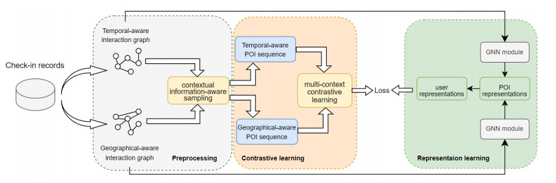
This paper focused on the point-of-interest (POI) recommendation task. Recently, graph representation learning-based POI recommendation models have gained significant attention due to the powerful modeling capacity of graph structural data. Despite their effectiveness, we have found that recent methods struggle to effectively utilize information from POIs that have not been checked in, which could limit their performance. Hence, in this paper, we proposed a new model, named the multi-contextual graph contrastive learning (MCGCL) model, which introduces the contrastive learning into graph representation learning-based methods. First, MCGCL extracts interactions between POIs under different contextual factors from user check-in records using predefined graph structure information. Next, it samples important POI sets from different contextual factors using a random walk-based method. Then, it introduces a new contrastive learning loss that incorporates contextual information into traditional contrastive learning to enhance its ability to capture contextual information. Finally, MCGCL employs a graph neural network (GNN) model to learn representations of users and POIs. Extensive experiments on real-world datasets have demonstrated the effectiveness of MCGCL on the POI recommendation task compared to representative POI recommendation approaches.

| [1] |
Y. Hwangbo, K. J. Lee, B. Jeong, K. Y. Park, Recommendation system with minimized transaction data, Data Sci. Manage., 4 (2021), 40-45. https://doi.org/10.1016/j.dsm.2022.01.001 doi: 10.1016/j.dsm.2022.01.001

|
| [2] |
L. Shi, G. Song, G. Cheng, X. Liu, A user-based aggregation topic model for understanding user's preference and intention in social network, Neurocomputing, 413 (2020), 1-13. https://doi.org/10.1016/j.neucom.2020.06.099 doi: 10.1016/j.neucom.2020.06.099
|
| [3] |
W. Ji, X. Meng, Y. Zhang, STARec: Adaptive learning with spatiotemporal and activity influence for POI recommendation, ACM Trans. Inf. Syst., 40 (2021), 1-40. https://doi.org/10.1145/3485631 doi: 10.1145/3485631
|
| [4] |
J. Wang, Z. Huang, Z. Liu, SQPMF: successive point of interest recommendation system based on probability matrix factorization, Appl. Intell., 54 (2024), 680-700. https://doi.org/10.1007/s10489-023-05196-x doi: 10.1007/s10489-023-05196-x
|
| [5] |
W. Ji, X. Meng, Y. Zhang, SPATM: A social period-aware topic model for personalized venue recommendation, IEEE Trans. Knowl. Data Eng., 34 (2020), 3997-4010. https://doi.org/10.1109/TKDE.2020.3029070 doi: 10.1109/TKDE.2020.3029070
|
| [6] |
F. Mo, X. Fan, C. Chen, H. Yamana, Sampling-based epoch differentiation calibrated graph convolution network for point-of-interest recommendation, Neurocomputing, 571 (2024), 127140. https://doi.org/10.1016/j.neucom.2023.127140 doi: 10.1016/j.neucom.2023.127140
|
| [7] |
X. Wang, D. Wang, D. Yu, R. Wu, Q. Yang, S. Deng, et al., Intent-aware graph neural network for point-of-interest embedding and recommendation, Neurocomputing, 557 (2023), 126734. https://doi.org/10.1016/j.neucom.2023.126734 doi: 10.1016/j.neucom.2023.126734
|
| [8] |
M. Gan, Y. Ma, Mapping user interest into hyper-spherical space: a novel poi recommendation method, Inf. Process. Manage., 60 (2023), 103169. https://doi.org/10.1016/j.ipm.2022.103169 doi: 10.1016/j.ipm.2022.103169
|
| [9] |
Y. Qin, C. Gao, Y. Wang, S. Wei, D. Jin, J. Yuan, et al., Disentangling geographical effect for point-of-interest recommendation, IEEE Trans. Knowl. Data Eng., 35 (2023), 7883-7897. https://doi.org/10.1109/TKDE.2022.3221873 doi: 10.1109/TKDE.2022.3221873
|
| [10] |
L. Shi, J. Luo, C. Zhu, F. Kou, G. Cheng, X. Liu, A survey on cross-media search based on user intention understanding in social networks, Inf. Fusion, 91 (2023), 566-581. https://doi.org/10.1016/j.inffus.2022.11.017 doi: 10.1016/j.inffus.2022.11.017
|
| [11] |
L. Shi, J. P. Du, G. Cheng, X. Liu, Z. G. Xiong, J. Luo, Cross‐media search method based on complementary attention and generative adversarial network for social networks, Int. J. Intell. Syst., 37 (2022), 4393-4416. https://doi.org/10.1002/int.22723 doi: 10.1002/int.22723
|
| [12] |
Z. Cai, G. Yuan, S. Qiao, S. Qu, Y. Zhang, R. Bing, FG-CF: Friends-aware graph collaborative filtering for POI recommendation, Neurocomputing, 488 (2022), 107-119. https://doi.org/10.1016/j.neucom.2022.02.070 doi: 10.1016/j.neucom.2022.02.070
|
| [13] |
Y. C. Chen, T. Thaipisutikul, T. K. Shih, A learning-based POI recommendation with spatiotemporal context awareness, IEEE Trans. Cybern., 52 (2020), 2453-2466. https://doi.org/10.1109/TCYB.2020.3000733 doi: 10.1109/TCYB.2020.3000733
|
| [14] |
C. Lang, Z. Wang, K. He, S. Sun, POI recommendation based on a multiple bipartite graph network model, J. Supercomput., 78 (2022), 9782-9816. https://doi.org/10.1007/s11227-021-04279-1 doi: 10.1007/s11227-021-04279-1
|
| [15] |
L. Chang, W. Chen, J. Huang, C. Bin, W. Wang, Exploiting multi-attention network with contextual influence for point-of-interest recommendation, Appl. Intell., 51 (2021), 1904-1917. https://doi.org/10.1007/s10489-020-01868-0 doi: 10.1007/s10489-020-01868-0
|
| [16] |
J. Zhang, X. Liu, X. Zhou, X. Chu, Leveraging graph neural networks for point-of-interest recommendations, Neurocomputing, 462 (2021), 1-13. https://doi.org/10.1016/j.neucom.2021.07.063 doi: 10.1016/j.neucom.2021.07.063
|
| [17] | G. Christoforidis, P. Kefalas, A. N. Papadopoulos, Y. Manolopoulos, RELINE: point-of-interest recommendations using multiple network embeddings, Knowl. Inf. Syst., 63 (2021), 791-817. |
| [18] | Y. Yang, Z. Wu, L. Wu, K. Zhang, R. Hong, Z. Zhang, et al., Generative-contrastive graph learning for recommendation, in Proceedings of the 46th International ACM SIGIR Conference on Research and Development in Information Retrieval, (2023), 1117-1126. https://doi.org/10.1145/3539618.3591691 |
| [19] |
L. Guo, J. Zhang, L. Tang, T. Chen, L. Zhu, H. Yin, Time interval-enhanced graph neural network for shared-account cross-domain sequential recommendation, IEEE Trans. Neural Networks Learn. Syst., 35 (2024), 4002-4016. https://doi.org/10.1109/TNNLS.2022.3201533 doi: 10.1109/TNNLS.2022.3201533
|
| [20] |
R. Gao, Y. Tao, Y. Yu, J. Wu, X. Shao, J. Li, et al., Self-supervised dual hypergraph learning with intent disentanglement for session-based recommendation, Knowl. Based Syst., 270 (2023), 110528. https://doi.org/10.1016/j.knosys.2023.110528 doi: 10.1016/j.knosys.2023.110528
|
| [21] |
C. Yang, J. Zou, J. Wu, H. Xu, S. Fan, Supervised contrastive learning for recommendation, Knowl. Based Syst., 258 (2022), 109973. https://doi.org/10.1016/j.knosys.2022.109973 doi: 10.1016/j.knosys.2022.109973
|
| [22] |
F. Wang, X. Lu, L. Lyu, CGSNet: Contrastive graph self-attention network for session-based recommendation, Knowl. Based Syst., 251 (2022), 109282. https://doi.org/10.1016/j.knosys.2022.109282 doi: 10.1016/j.knosys.2022.109282
|
| [23] |
Q. Li, H. Ma, R. Zhang, W. Jin, Z. Li, Dual-view co-contrastive learning for multi-behavior recommendation, Appl. Intell., 53 (2023), 20134-20151. https://doi.org/10.1007/s10489-023-04495-7 doi: 10.1007/s10489-023-04495-7
|
| [24] |
Y. Zhang, G. Yin, Y. Dong, L. Zhang, Contrastive learning with frequency domain for sequential recommendation, Appl. Soft Comput., 144 (2023), 110481. https://doi.org/10.1016/j.asoc.2023.110481 doi: 10.1016/j.asoc.2023.110481
|
| [25] |
S. Xiao, D. Zhu, C. Tang, Z. Huang, Combining graph contrastive embedding and multi-head cross-attention transfer for cross-domain recommendation, Data Sci. Eng., 8 (2023), 247-262. https://doi.org/10.1007/s41019-023-00226-7 doi: 10.1007/s41019-023-00226-7
|
| [26] |
Y. He, G. Wu, D. Cai, X. Hu, Meta-path based graph contrastive learning for micro-video recommendation, Expert Syst. Appl., 222 (2023), 119713. https://doi.org/10.1016/j.eswa.2023.119713 doi: 10.1016/j.eswa.2023.119713
|
| [27] |
J. Ji, B. Zhang, J. Yu, X. Zhang, D. Qiu, B. Zhang, Relationship-aware contrastive learning for social recommendations, Inf. Sci., 629 (2023), 778-797. https://doi.org/10.1016/j.ins.2023.02.011 doi: 10.1016/j.ins.2023.02.011
|
| [28] |
H. Tang, G. Zhao, Y. He, Y. Wu, X. Qian, Ranking-based contrastive loss for recommendation systems, Knowl. Based Syst., 261 (2023), 110180. https://doi.org/10.1016/j.knosys.2022.110180 doi: 10.1016/j.knosys.2022.110180
|
| [29] |
J. Zhuang, S. Meng, J. Zhang, V. S. Sheng, Contrastive learning based graph convolution network for social recommendation, ACM Trans. Knowl. Discov. Data, 17 (2023), 1-21. https://doi.org/10.1145/3587268 doi: 10.1145/3587268
|
| [30] | Y. Qin, Y. Wang, F. Sun, W. Ju, X. Hou, Z. Wang, et al., DisenPOI: Disentangling sequential and geographical influence for point-of-interest recommendation, in Proceedings of the Sixteenth ACM International Conference on Web Search and Data Mining, (2023), 508-516. https://doi.org/10.1145/3539597.3570408 |
| [31] | W. Ju, Y. Qin, Z. Qiao, X. Luo, Y. Wang, Y. Fu, et al., Kernel-based substructure exploration for next POI recommendation, in Proceedings of the 2022 IEEE International Conference on Data Mining, (2022), 221-230. https://doi.org/10.1109/ICDM54844.2022.00032 |
| [32] | J. D. Zhang, C. Y. Chow, Geosoca: Exploiting geographical, social and categorical correlations for point-of-interest recommendations, in Proceedings of the 38th International ACM SIGIR Conference on Research and Development in Information Retrieval, (2015), 443-452. https://doi.org/10.1145/2766462.2767711 |
| [33] | S. Feng, G. Cong, B. An, Y. M. Chee, Poi2vec: Geographical latent representation for predicting future visitors, in Proceedings of the AAAI Conference on Artificial Intelligence, (2017), 102-108. https://doi.org/10.1609/aaai.v31i1.10500 |
| [34] |
P. Zhao, A. Luo, Y. Liu, J. Xu, Z. Li, F. Zhuang, et al., Where to go next: A spatio-temporal gated network for next poi recommendation, IEEE Trans. Knowl. Data Eng., 34 (2022), 2512-2524. https://doi.org/10.1109/TKDE.2020.3007194 doi: 10.1109/TKDE.2020.3007194
|
| [35] | B. Chang, G. Jang, S. Kim, J. Kang, Learning graph-based geographical latent representation for point-of-interest recommendation, in Proceedings of the 29th ACM International Conference on Information & Knowledge Management, (2020), 135-144. https://doi.org/10.1145/3340531.3411905 |
| [36] |
Z. Wang, Y. Zhu, Q. Zhang, H. Liu, C. Wang, T. Liu, Graph-enhanced spatial-temporal network for next POI recommendation, ACM Trans. Knowl. Discov. Data, 16 (2022), 1-21. https://doi.org/10.1145/3513092 doi: 10.1145/3513092
|
| [37] | Q. Liu, S. Wu, L. Wang, T. Tan, Predicting the next location: A recurrent model with spatial and temporal contexts, in Proceedings of the AAAI Conference on Artificial Intelligence, (2016), 194-200. https://doi.org/10.1609/aaai.v30i1.9971 |
| [38] |
J. Fu, R. Gao, Y. Yu, J. Wu, J. Li, D. Liu, et al., Contrastive graph learning long and short-term interests for POI recommendation, Expert Syst. Appl., 238 (2024), 121931. https://doi.org/10.1016/j.eswa.2023.121931 doi: 10.1016/j.eswa.2023.121931
|
| [39] |
M. Acharya, K. K. Mohbey, D. S. Rajput, Long-term preference mining with temporal and spatial fusion for point-of-interest recommendation, IEEE Access, 12 (2024), 11584-11596. https://doi.org/10.1109/ACCESS.2024.3354934 doi: 10.1109/ACCESS.2024.3354934
|


Figures(5) / Tables(10)
Xueping Han, Xueyong Wang. MCGCL: A multi-contextual graph contrastive learning-based approach for POI recommendation[J]. Electronic Research Archive, 2024, 32(5): 3618-3634. doi: 10.3934/era.2024166


 DownLoad: