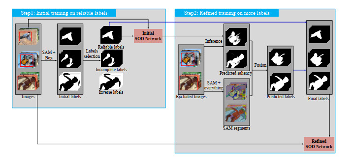
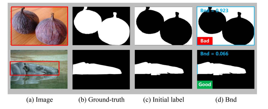
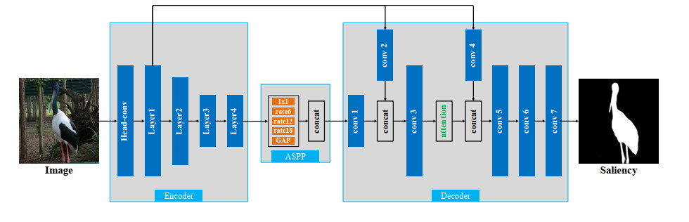
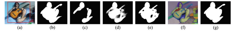
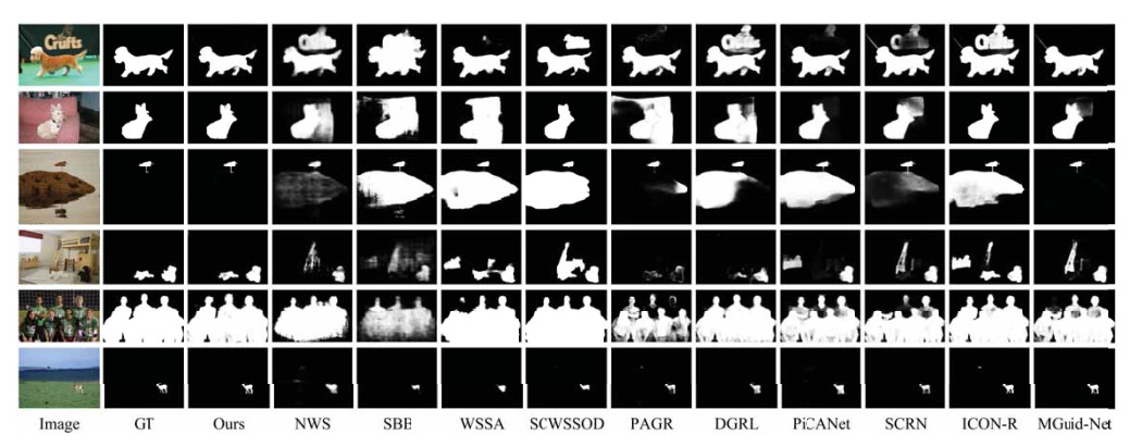
Salient object detection (SOD) aims to detect the most attractive region in an image. Fully supervised SOD based on deep learning usually needs a large amount of data with human annotation. Researchers have gradually focused on the SOD task using weakly supervised annotation such as category, scribble, and bounding-box, while these existing weakly supervised methods achieve limited performance and demonstrate a huge performance gap with fully supervised methods. In this work, we proposed one novel two-stage weakly supervised method based on bounding-box annotation and the recent large visual model Segment Anything (SAM). In the first stage, we regarded the bounding-box annotation as the box prompt of SAM to generate initial labels and proposed object completeness check and object inversion check to exclude low quality labels, then we selected reliable pseudo labels for the training initial SOD model. In the second stage, we used the initial SOD model to predict the saliency map of excluded images and adopted SAM with the everything mode to generate segmentation candidates, then we fused the saliency map and segmentation candidates to predict pseudo labels. Finally we used all reliable pseudo labels generated in the two stages to train one refined SOD model. We also designed a simple but effective SOD model, which can capture rich global context information. Performance evaluation on four public datasets showed that the proposed method significantly outperforms other weakly supervised methods and also achieves comparable performance with fully supervised methods.
Citation: Xiangquan Liu, Xiaoming Huang. Weakly supervised salient object detection via bounding-box annotation and SAM model[J]. Electronic Research Archive, 2024, 32(3): 1624-1645. doi: 10.3934/era.2024074
Salient object detection (SOD) aims to detect the most attractive region in an image. Fully supervised SOD based on deep learning usually needs a large amount of data with human annotation. Researchers have gradually focused on the SOD task using weakly supervised annotation such as category, scribble, and bounding-box, while these existing weakly supervised methods achieve limited performance and demonstrate a huge performance gap with fully supervised methods. In this work, we proposed one novel two-stage weakly supervised method based on bounding-box annotation and the recent large visual model Segment Anything (SAM). In the first stage, we regarded the bounding-box annotation as the box prompt of SAM to generate initial labels and proposed object completeness check and object inversion check to exclude low quality labels, then we selected reliable pseudo labels for the training initial SOD model. In the second stage, we used the initial SOD model to predict the saliency map of excluded images and adopted SAM with the everything mode to generate segmentation candidates, then we fused the saliency map and segmentation candidates to predict pseudo labels. Finally we used all reliable pseudo labels generated in the two stages to train one refined SOD model. We also designed a simple but effective SOD model, which can capture rich global context information. Performance evaluation on four public datasets showed that the proposed method significantly outperforms other weakly supervised methods and also achieves comparable performance with fully supervised methods.

| [1] | J. Redmon, S. Divvala, R. Girshick, A. Farhadi, You only look once: Unified, real-time object detection, in 2016 IEEE Conference on Computer Vision and Pattern Recognition (CVPR), (2016), 779–788. https://doi.org/10.1109/CVPR.2016.91 |
| [2] |
X. Yang, X. Qian, Y. Xue, Scalable mobile image retrieval by exploring contextual saliency, IEEE Trans. Image Process., 24 (2015), 1709–1721. https://doi.org/10.1109/TIP.2015.2411433 doi: 10.1109/TIP.2015.2411433

|
| [3] |
Y. Su, Q. Zhao, L. Zhao, D. Gu, Abrupt motion tracking using a visual saliency embedded particle filter, Pattern Recognit., 47 (2014), 1826–1834. https://doi.org/10.1016/j.patcog.2013.11.028 doi: 10.1016/j.patcog.2013.11.028
|
| [4] | X. Huang, Y. Zhang, 300-fps salient object detection via minimum directional contrast, IEEE Trans. Image Process., 26 (2017). 4243–4254, https://doi.org/10.1109/TIP.2017.2710636 |
| [5] |
X. Huang, Y. Zhang, Water flow driven salient object detection at 180 fps, Pattern Recognit., 76 (2018), 95–107. https://doi.org/10.1016/j.patcog.2017.10.027 doi: 10.1016/j.patcog.2017.10.027
|
| [6] |
X. Huang, Y. Zheng, J. Huang, Y. Zhang, 50 fps object-level saliency detection via maximally stable region, IEEE Trans. Image Process., 29 (2020), 1384–1396. https://doi.org/10.1109/TIP.2019.2941663 doi: 10.1109/TIP.2019.2941663
|
| [7] |
M. Cheng, N. J. Mitra, X. Huang, P. H. S. Torr, S. Hu, Global contrast based salient region detection, IEEE Trans. Pattern Anal. Mach. Intell., 37 (2015), 569–582. https://doi.org/10.1109/TPAMI.2014.2345401 doi: 10.1109/TPAMI.2014.2345401
|
| [8] | C. Yang, L. Zhang, H. Lu, X. Ruan, M. Yang, Saliency detection via graph-based manifold ranking, in 2013 IEEE Conference on Computer Vision and Pattern Recognition, (2013), 3166–3173. https://doi.org/10.1109/CVPR.2013.407 |
| [9] | Z. Wu, L. Su, Q. Huang, Stacked cross refinement network for edge-aware salient object detection, in 2019 IEEE/CVF International Conference on Computer Vision (ICCV), (2019), 7263–7272. https://doi.org/10.1109/ICCV.2019.00736 |
| [10] | N. Liu, N. Zhang, K. Wan, L. Shao, J. Han, Visual saliency transformer, in 2021 IEEE/CVF International Conference on Computer Vision (ICCV), (2021), 4722–4732. https://doi.org/10.1109/ICCV48922.2021.00468 |
| [11] |
J. Liu, Q. Hou, Z. Liu, M. Cheng, PoolNet+: Exploring the potential of pooling for salient object detection, IEEE Trans. Pattern Anal. Mach. Intell., 45 (2023), 887–904. https://doi.org/10.1109/TPAMI.2021.3140168 doi: 10.1109/TPAMI.2021.3140168
|
| [12] |
M. Zhuge, D. Fan, N. Liu, D. Zhang, D. Xu, L. Shao, Salient object detection via integrity learning, IEEE Trans. Pattern Anal. Mach. Intell., 45 (2023), 3738–3752. https://doi.org/10.1109/TPAMI.2022.3179526 doi: 10.1109/TPAMI.2022.3179526
|
| [13] |
S. Hui, Q. Guo, X. Geng, C. Zhang, Multi-guidance cnns for salient object detection, ACM Trans. Multimedia Comput. Commun. Appl., 19 (2023), 1–19. https://doi.org/10.1145/3570507 doi: 10.1145/3570507
|
| [14] | G. Li, Y. Xie, L. Lin, Weakly supervised salient object detection using image labels, in Thirty-Second AAAI Conference on Artificial Intelligence, 32 (2018), 7024–7031. https://doi.org/10.1609/aaai.v32i1.12308 |
| [15] | L. Wang, H. Lu, Y. Wang, M. Feng, D. Wang, B. Yin, et al., Learning to detect salient objects with image-level supervision, in 2017 IEEE Conference on Computer Vision and Pattern Recognition (CVPR), (2017), 3796–3805. https://doi.org/10.1109/CVPR.2017.404 |
| [16] | Y. Piao, J. Wang, M. Zhang, H. Lu, Mfnet: Multi-filter directive network for weakly supervised salient object detection, in 2021 IEEE/CVF International Conference on Computer Vision (ICCV), (2021), 4116–4125. https://doi.org/10.1109/ICCV48922.2021.00410 |
| [17] |
Y. Piao, W. Wu, M. Zhang, Y. Jiang, H. Lu, Noise-sensitive adversarial learning for weakly supervised salient object detection, IEEE Trans. Multimedia, 25 (2023), 2888–2897. https://doi.org/10.1109/TMM.2022.3152567 doi: 10.1109/TMM.2022.3152567
|
| [18] | J. Zhang, X. Yu, A. Li, P. Song, B. Liu, Y. Dai, Weakly-supervised salient object detection via scribble annotations, in 2020 IEEE/CVF Conference on Computer Vision and Pattern Recognition (CVPR), (2020), 12543–12552. https://doi.org/10.1109/CVPR42600.2020.01256 |
| [19] | S. Yu, B. Zhang, J. Xiao, E. G. Lim, Structure-consistent weakly supervised salient object detection with local saliency coherence, in AAAI Conference on Artificial Intelligence, (2021), 3234–3242. https://doi.org/10.1609/aaai.v35i4.16434 |
| [20] | J. Dai, K. He, J. Sun, Boxsup: Exploiting bounding boxes to supervise convolutional networks for semantic segmentation, in 2015 IEEE International Conference on Computer Vision (ICCV), (2015), 1635–1643. https://doi.org/10.1109/ICCV.2015.191 |
| [21] | A. Khoreva, R. Benenson, J. Hosang, M. Hein, B. Schiele, Simple does it: Weakly supervised instance and semantic segmentation, in 2017 IEEE Conference on Computer Vision and Pattern Recognition (CVPR), (2017), 1665–1674. https://doi.org/10.1109/CVPR.2017.181 |
| [22] | Q. Wang, X. Huang, Q. Tong, X. Liu, Weakly supervised salient object detection algorithm based on bounding box annotation, J. Comput. Appl., 43 (2023), 1910–1918. |
| [23] |
C. Rother, V. Kolmogorov, A. Blake, "GrabCut": Interactive foreground extraction using iterated graph cuts, ACM Trans. Graphics, 23 (2004), 309–314. https://doi.org/10.1145/1015706.1015720 doi: 10.1145/1015706.1015720
|
| [24] | A. Kirillov, E. Mintun, N. Ravi, H. Mao, C. Rolland, L. Gustafson, et al., Segment anything, preprint, arXiv: 2304.02643. |
| [25] |
Y. Liu, P. Wang, Y. Cao, Z. Liang, R. W. H. Lau, Weakly-supervised salient object detection with saliency bounding boxes, IEEE Trans. Image Process., 30 (2021), 4423–4435. https://doi.org/10.1109/TIP.2021.3071691 doi: 10.1109/TIP.2021.3071691
|
| [26] | Y. Zeng, Y. Zhuge, H. Lu, L. Zhang, M. Qian, Y. Yu, Multi-source weak supervision for saliency detection, in 2019 IEEE/CVF Conference on Computer Vision and Pattern Recognition (CVPR), (2019), 6067–6076. https://doi.org/10.1109/CVPR.2019.00623 |
| [27] |
J. Lu, L. Pan, J. Deng, H. Chai, Z. Ren, Y. Shi, Deep learning for flight maneuver recognition: A survey, Electron. Res. Arch., 31 (2023), 75–102. https://doi.org/10.3934/era.2023005 doi: 10.3934/era.2023005
|
| [28] |
Z. Feng, K. Qi, B. Shi, H. Mei, Q. Zheng, H. Wei, Deep evidential learning in diffusion convolutional recurrent neural network, Electron. Res. Arch., 31 (2023), 2252–2264. https://doi.org/10.3934/era.2023115 doi: 10.3934/era.2023115
|
| [29] |
J. Wang, L. Zhang, S. Yang, S. Lian, P. Wang, L. Yu, et al., Optimized LSTM based on improved whale algorithm for surface subsidence deformation prediction, Electron. Res. Arch., 31 (2023), 3435–3452. https://doi.org/10.3934/era.2023174 doi: 10.3934/era.2023174
|
| [30] |
C. Swarup, K. U. Singh, A. Kumar, S. K. Pandey, N. varshney, T. Singh, Brain tumor detection using CNN, AlexNet & GoogLeNet ensembling learning approaches, Electron. Res. Arch., 31 (2023), 2900–2924. https://doi.org/10.3934/era.2023146 doi: 10.3934/era.2023146
|
| [31] |
R. Bi, L. Guo, B. Yang, J. Wang, C. Shi, 2.5D cascaded context-based network for liver and tumor segmentation from CT images, Electron. Res. Arch., 31 (2023), 4324–4345. https://doi.org/10.3934/era.2023221 doi: 10.3934/era.2023221
|
| [32] | S. Kara, H. Ammar, F. Chabot, Q. Pham, Image segmentation-based unsupervised multiple objects discovery, in 2023 IEEE/CVF Winter Conference on Applications of Computer Vision (WACV), (2023), 3276–3285. https://doi.org/10.1109/WACV56688.2023.00329 |
| [33] | T. Chen, Z. Mai, R. Li, W. Chao, Segment anything model (SAM) enhanced pseudo labels for weakly supervised semantic segmentation, preprint, arXiv: 2305.05803. |
| [34] | H. Yamagiwa, Y. Takase, H. Kambe, R. Nakamoto, Zero-shot edge detection with SCESAME: Spectral clustering-based ensemble for segment anything model estimation, preprint, arXiv: 2308.13779. |
| [35] | R. Zhang, Z. Jiang, Z. Guo, S. Yan, J. Pan, X. Ma, et al., Personalize segment anything model with one shot, preprint, arXiv: 2305.03048. |
| [36] | T. Chen, L. Zhu, C. Ding, R. Cao, Y. Wang, Z. Li, et al., SAM fails to segment anything?–SAM-adapter: Adapting SAM in underperformed scenes: Camouflage, shadow, and more, preprint, arXiv: 2304.09148. |
| [37] | X. Zhao, W. Ding, Y. An, Y. Du, T. Yu, M. Li, et al., Fast segment anything, preprint, arXiv: 2306.12156. |
| [38] | H. Li, G. Chen, G. Li, Y. Yu, Motion guided attention for video salient object detection, in 2019 IEEE/CVF International Conference on Computer Vision (ICCV), (2019), 7273–7282. https://doi.org/10.1109/ICCV.2019.00737 |
| [39] | K. He, X. Zhang, S. Ren, J. Sun, Deep residual learning for image recognition, in 2016 IEEE Conference on Computer Vision and Pattern Recognition (CVPR), (2016), 770–778. https://doi.org/10.1109/CVPR.2016.90 |
| [40] | F. Deng, H. Feng, M. Liang, H. Wang, Y. Yang, Y. Gao, et al., FEANet: Feature-enhanced attention network for RGB-thermal real-time semantic segmentation, in 2021 IEEE/RSJ International Conference on Intelligent Robots and Systems (IROS), (2021), 4467–4473. https://doi.org/10.1109/IROS51168.2021.9636084 |
| [41] | J. Deng, W. Dong, R. Socher, L. Li, K. Li, L. Fei-Fei, Imagenet: A large-scale hierarchical image database, in 2009 IEEE Conference on Computer Vision and Pattern Recognition, (2009), 248–255. https://doi.org/10.1109/CVPR.2009.5206848 |
| [42] | Q. Yan, L. Xu, J. Shi, J. Jia, Hierarchical saliency detection, in 2013 IEEE Conference on Computer Vision and Pattern Recognition, (2013), 1155–1162. https://doi.org/10.1109/CVPR.2013.153 |
| [43] |
G. Li, Y. Yu, Visual saliency detection based on multiscale deep CNN features, IEEE Trans. Image Process., 25 (2016), 5012–5024. https://doi.org/10.1109/TIP.2016.2602079 doi: 10.1109/TIP.2016.2602079
|
| [44] | X. Zhang, T. Wang, J. Qi, H. Lu, G. Wang, Progressive attention guided recurrent network for salient object detection, in 2018 IEEE/CVF Conference on Computer Vision and Pattern Recognition, (2018), 714–722. https://doi.org/10.1109/CVPR.2018.00081 |
| [45] | L. Zhang, J. Dai, H. Lu, Y. He, G. Wang, A bi-directional message passing model for salient object detection, in 2018 IEEE/CVF Conference on Computer Vision and Pattern Recognition, (2018), 1741–1750. https://doi.org/10.1109/CVPR.2018.00187 |
| [46] | T. Wang, L. Zhang, S. Wang, H. Lu, G. Yang, X. Ruan, et al., Detect globally, refine locally: A novel approach to saliency detection, in 2018 IEEE/CVF Conference on Computer Vision and Pattern Recognition, (2018), 3127–3135. https://doi.org/10.1109/CVPR.2018.00330 |
| [47] | N. Liu, J. Han, M. Yang, PiCANet: Learning pixel-wise contextual attention for saliency detection, in 2018 IEEE/CVF Conference on Computer Vision and Pattern Recognition, (2018), 3089–3098. https://doi.org/10.1109/CVPR.2018.00326 |
| [48] | H. Zhou, B. Qiao, L. Yang, J. Lai, X. Xie, Texture-guided saliency distilling for unsupervised salient object detection, in 2023 IEEE/CVF Conference on Computer Vision and Pattern Recognition (CVPR), (2023), 7257–7267. http://doi.org/10.1109/cvpr52729.2023.00701 |
| [49] | Y. Wang, W. Zhang, L. Wang, T. Liu, H. Lu, Multi-source uncertainty mining for deep unsupervised saliency detection, in 2022 IEEE/CVF Conference on Computer Vision and Pattern Recognition (CVPR), (2022), 11717–11726. https://doi.org/10.1109/CVPR52688.2022.01143 |
| [50] | P. Yan, Z. Wu, M. Liu, K. Zeng, L. Lin, G. Li, Unsupervised domain adaptive salient object detection through uncertainty-aware pseudo-label learning, in AAAI Conference on Artificial Intelligence, (2022), 3000–3008. https://doi.org/10.1609/aaai.v36i3.20206 |
| [51] | A. Voynov, S. Morozov, A. Babenko, Object segmentation without labels with large-scale generative models, preprint, arXiv: 2006.04988. |
| [52] |
S. Jardim, J. António, C. Mora, Graphical image region extraction with k-means clustering and watershed, J. Imaging, 8 (2022), 163. https://doi.org/10.3390/jimaging8060163 doi: 10.3390/jimaging8060163
|
| [53] |
G. Li, Z. Liu, D. Zeng, W. Lin, H. Ling, Adjacent context coordination network for salient object detection in optical remote sensing images, IEEE Trans. Cybern., 53 (2023), 526–538. https://doi.org/10.1109/TCYB.2022.3162945 doi: 10.1109/TCYB.2022.3162945
|
| [54] |
G. Li, Z. Liu, Z. Bai, W. Lin, H. Ling, Lightweight salient object detection in optical remote sensing images via feature correlation, IEEE Trans. Geosci. Remote Sens., 60 (2022), 1–12. https://doi.org/10.1109/TGRS.2022.3145483 doi: 10.1109/TGRS.2022.3145483
|
| [55] |
G. Li, Z. Bai, Z. Liu, X. Zhang, H. Ling, Salient object detection in optical remote sensing images driven by transformer, IEEE Trans. Image Process., 32 (2023), 5257–5269. https://doi.org/10.1109/TIP.2023.3314285 doi: 10.1109/TIP.2023.3314285
|
Figures(8) / Tables(8)
Xiangquan Liu, Xiaoming Huang. Weakly supervised salient object detection via bounding-box annotation and SAM model[J]. Electronic Research Archive, 2024, 32(3): 1624-1645. doi: 10.3934/era.2024074


 DownLoad: