Multitudinous potential homoclinic and heteroclinic orbits seized

Haijun Wang; Jun Pan; Guiyao Ke; Haijun Wang; Jun Pan; Guiyao Ke

doi:10.3934/era.2024049

Electronic Research Archive

2024, Volume 32, Issue 2: 1003-1016. doi: 10.3934/era.2024049

Previous Article Next Article

Research article

Multitudinous potential homoclinic and heteroclinic orbits seized

Haijun Wang ¹,
Jun Pan ^{2
,
,},
Guiyao Ke ^{3,4,5
,
,}

1.
School of Electronic and Information Engineering (School of Big Data Science), Taizhou University, Taizhou, 318000, China
2.
Department of Big Data Science, School of Science, Zhejiang University of Science and Technology, Hangzhou 310023, China
3.
School of Information, Zhejiang Guangsha Vocational and Technical University of Construction, Dongyang, Zhejiang 322100, China
4.
HUIKE Education Technology Group Co., Ltd., China
5.
School of Information Engineering, GongQing Institute of Science and Technology, Gongqingcheng 332020, China

Received: 04 October 2023 Revised: 10 November 2023 Accepted: 16 November 2023 Published: 19 January 2024

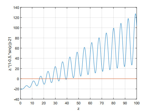
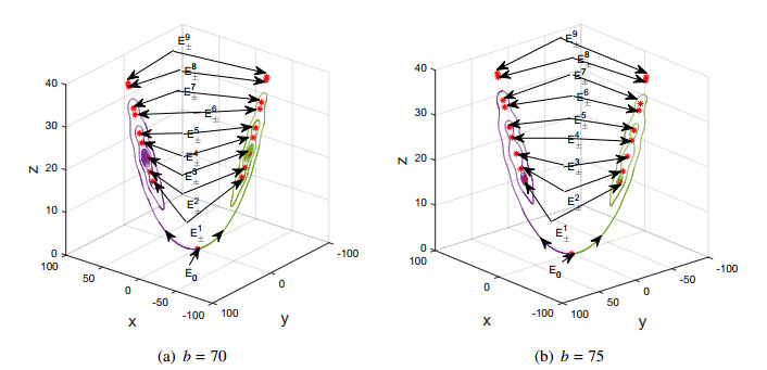
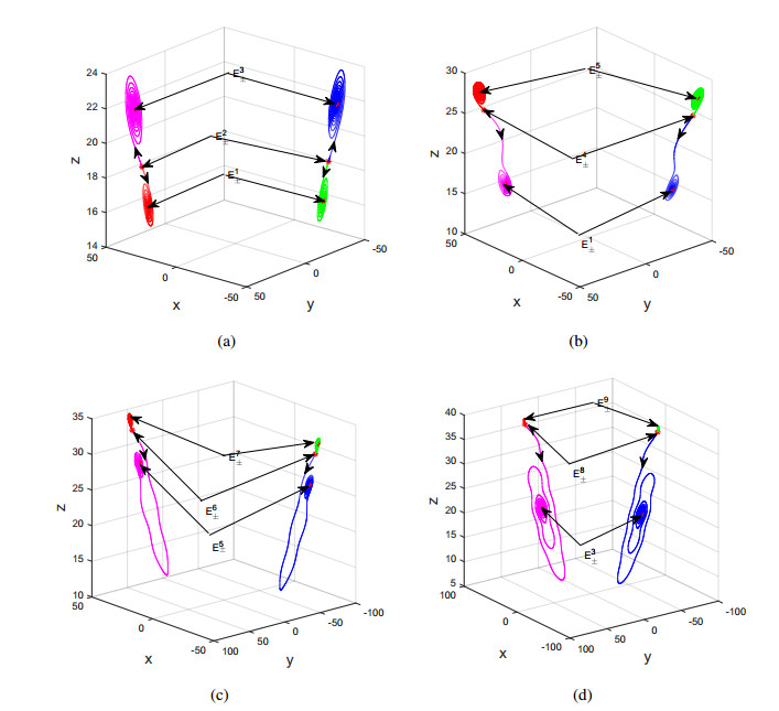
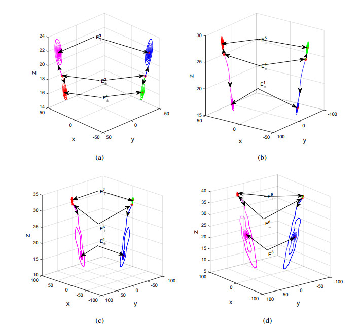
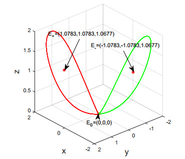
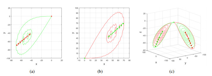
Revisiting a newly reported modified Chen system by both the definitions of $ \alpha $-limit and $ \omega $-limit set, Lyapunov function and Hamiltonian function, this paper seized a multitude of pairs of potential heteroclinic orbits to (1) $ E_{0} $ and $ E_{\pm} $, or (2) $ E_{+} $ or (3) $ E_{-} $, and homoclinic and heteroclinic orbits on its invariant algebraic surface $ Q = z - \frac{x^{2}}{2a} = 0 $ with cofactor $ -2a $, which is not available in the existing literature to the best of our knowledge. Particularly, the theoretical conclusions were verified via numerical examples.
- new 3D modified Chen system,
- multi-wing chaotic attractor,
- homoclinic and heteroclinic orbit,
- Lyapunov function
Citation: Haijun Wang, Jun Pan, Guiyao Ke. Multitudinous potential homoclinic and heteroclinic orbits seized[J]. Electronic Research Archive, 2024, 32(2): 1003-1016. doi: 10.3934/era.2024049

Related Papers:

Abstract

Revisiting a newly reported modified Chen system by both the definitions of $ \alpha $-limit and $ \omega $-limit set, Lyapunov function and Hamiltonian function, this paper seized a multitude of pairs of potential heteroclinic orbits to (1) $ E_{0} $ and $ E_{\pm} $, or (2) $ E_{+} $ or (3) $ E_{-} $, and homoclinic and heteroclinic orbits on its invariant algebraic surface $ Q = z - \frac{x^{2}}{2a} = 0 $ with cofactor $ -2a $, which is not available in the existing literature to the best of our knowledge. Particularly, the theoretical conclusions were verified via numerical examples.

References

[1]	S. Sahoo, B. K. Roy, Design of multi-wing chaotic systems with higher largest Lyapunov exponent, Chaos, Solitons Fractals, 157 (2022), 111926. https://doi.org/10.1016/j.chaos.2022.111926 doi: 10.1016/j.chaos.2022.111926
[2]	E. Freire, A. J. Rodriguez-Luis, E. Gamero, E. Ponce, A case study for homoclinic chaos in an autonomous electronic circuit: A trip from Takens-Bogdanov to Hopf-Šil'nikov, Physica D, 62 (1993), 230–253. https://doi.org/10.1016/0167-2789(93)90284-8 doi: 10.1016/0167-2789(93)90284-8
[3]	P. Glendinning, C. Sparrow, Local and global behaviour near homoclinic orbits, J. Stat. Phys., 35 (1984), 645–696. https://doi.org/10.1007/BF01010828 doi: 10.1007/BF01010828
[4]	G. W. Hunt, M. A. Peletier, A. R. Champneys, P. D. Woods, M. Ahmerwaddee, C. J. Budd, et al., Cellular buckling in long structures, Nonlinear Dyn., 21 (2000), 3–29. https://doi.org/10.1023/A:1008398006403 doi: 10.1023/A:1008398006403
[5]	B. Aulbach, D. Flockerzi, The past in short hypercycles, J. Math. Biol., 27 (1989), 223–231. https://doi.org/10.1007/BF00276104 doi: 10.1007/BF00276104
[6]	N. J. Balmforth, Solitary waves and homoclinic orbits, Annu. Rev. Fluid Mech., 27 (1995), 335–373. https://doi.org/10.1146/annurev.fl.27.010195.002003 doi: 10.1146/annurev.fl.27.010195.002003
[7]	R. M. May, W. Leonard, Nonlinear aspect of competition between three species, SIAM J. Appl. Math., 29 (1975), 243–253. https://doi.org/10.1137/0129022 doi: 10.1137/0129022
[8]	J. Hofbauer, K. Sigmund, On the stabilizing effect of predator and competitors on ecological communities, J. Math. Biol., 27 (1975), 537–548. https://doi.org/10.1007/BF00288433 doi: 10.1007/BF00288433
[9]	B. Y. Feng, The heteroclinic cycle in the model of competition between n species and its stability, Acta Math. Appl. Sin., 14 (1998), 404–413. https://doi.org/10.1007/BF02683825 doi: 10.1007/BF02683825
[10]	W. S. Koon, M. W. Lo, J. E. Marsden, S. D. Ross, Heteroclinic connections between periodic orbits and resonance transitions in celestial mechanics, Chaos, 10 (2000), 427–469. https://doi.org/10.1063/1.166509 doi: 10.1063/1.166509
[11]	D. Wilczak, P. Zgliczyński, Heteroclinic connections between periodic orbits in planar restricted circular three body problem-A computer assisted proof, Commun. Math. Phys., 234 (2003), 37–75. https://doi.org/10.1007/s00220-002-0709-0 doi: 10.1007/s00220-002-0709-0
[12]	D. Wilczak, P. Zgliczyński, Heteroclinic connections between periodic orbits in planar restricted circular three body problem. part Ⅱ, Commun. Math. Phys., 259 (2005), 561–576. https://doi.org/10.1007/s00220-005-1471-x doi: 10.1007/s00220-005-1471-x
[13]	S. Wiggins, Introduction to Applied Nonlinear Dynamical System and Chaos, 2nd edition, Springer, New York, 2003. https://doi.org/10.1007/978-1-4757-4067-7
[14]	L. P. Shilnikov, A. L. Shilnikov, D. V. Turaev, L. O. Chua, Methods of Qualitative Theory in Nonlinear Dynamics, Part II, World Scientific, Singapore, 2001. https://doi.org/10.1142/4221
[15]	T. Li, G. Chen, G. Chen, On homoclinic and heteroclinic orbits of the Chen's system, Int. J. Bifurcation Chaos, 16 (2006), 3035–3041. https://doi.org/10.1142/S021812740601663X doi: 10.1142/S021812740601663X
[16]	G. Tigan, J. Llibre, Heteroclinic, homoclinic and closed orbits in the Chen system, Int. J. Bifurcation Chaos, 26 (2016), 1650072. https://doi.org/10.1142/S0218127416500723 doi: 10.1142/S0218127416500723
[17]	H. Wang, X. Li, More dynamical properties revealed from a 3D Lorenz-like system, Int. J. Bifurcation Chaos, 24 (2014), 1450133. https://doi.org/10.1142/S0218127414501338 doi: 10.1142/S0218127414501338
[18]	H. Wang, X. Li, On singular orbits and a given conjecture for a 3D Lorenz-like system, Nonlinear Dyn., 80 (2015), 969–981. https://doi.org/10.1007/s11071-015-1921-8 doi: 10.1007/s11071-015-1921-8
[19]	H. Wang, X. Li, Infinitely many heteroclinic orbits of a complex Lorenz system, Int. J. Bifurcation Chaos, 27 (2017), 1750110. https://doi.org/10.1142/S0218127417501103 doi: 10.1142/S0218127417501103
[20]	H. Wang, X. Li, A novel hyperchaotic system with infinitely many heteroclinic orbits coined, Chaos, Solitons Fractals, 106 (2018), 5–15. https://doi.org/10.1016/j.chaos.2017.10.029 doi: 10.1016/j.chaos.2017.10.029
[21]	H. Wang, F. Zhang, Bifurcations, ultimate boundedness and singular orbits in a unified hyperchaotic Lorenz-type system, Discrete Contin. Dyn. Syst. Ser. B, 25 (2020), 1791–1820. https://doi.org/10.3934/dcdsb.2020003 doi: 10.3934/dcdsb.2020003
[22]	H. Wang, H. Fan, J. Pan, Complex dynamics of a four-dimensional circuit system, Int. J. Bifurcation Chaos, 31 (2021), 2150208. https://doi.org/10.1142/S0218127421502084 doi: 10.1142/S0218127421502084
[23]	H. Wang, G. Ke, J. Pan, F. Hu, H. Fan, Multitudinous potential hidden Lorenz-like attractors coined, Eur. Phys. J. Spec. Top., 231 (2022), 359–368. https://doi.org/10.1140/epjs/s11734-021-00423-3 doi: 10.1140/epjs/s11734-021-00423-3
[24]	H. Wang, G. Ke, J. Pan, F. Hu, H. Fan, Q. Su, Two pairs of heteroclinic orbits coined in a new sub-quadratic Lorenz-like system, Eur. Phys. J. B, 96 (2023), 1–9. https://doi.org/10.1140/epjb/s10051-023-00491-5 doi: 10.1140/epjb/s10051-023-00491-5
[25]	Z. Li, G. Ke, H. Wang, J. Pan, F. Hu, Q. Su, Complex dynamics of a sub-quadratic Lorenz-like system, Open Phys., 21 (2023), 20220251. https://doi.org/10.1515/phys-2022-0251 doi: 10.1515/phys-2022-0251
[26]	F. Tricomi, Integration of a differential equation presented in electrical engineering, Ann. Sc. Norm. Super. Pisa Cl. Sci., 2 (1933), 1–20.
[27]	G. A. Leonov, Fishing principle for homoclinic and heteroclinic trajectories, Nonlinear Dyn., 78 (2014), 2751–2758. https://doi.org/10.1007/s11071-014-1622-8 doi: 10.1007/s11071-014-1622-8
[28]	G. Tigan, D. Turaev, Analytical search for homoclinic bifurcations in the Shimizu-Morioka model, Physica D, 240 (2011), 985–989. https://doi.org/10.1016/j.physd.2011.02.013 doi: 10.1016/j.physd.2011.02.013
[29]	B. Feng, R. Hu, A survey on homoclinic and heteroclinic orbits, Appl. Math. E-Notes, 3 (2003), 16–37.
[30]	X. Zhang, G. Chen, Constructing an autonomous system with infinitely many chaotic attractors, Chaos, 27 (2017), 071101. https://doi.org/10.1063/1.4986356 doi: 10.1063/1.4986356
[31]	X. Zhang, Boundedness of a class of complex Lorenz systems, Int. J. Bifurcation Chaos, 31 (2021), 2150101. https://doi.org/10.1142/S0218127421501017 doi: 10.1142/S0218127421501017
[32]	H. E. Gilardi-Velázquez, R. J. Escalante-González, E. Campos, Emergence of a square chaotic attractor through the collision of heteroclinic orbits, Eur. Phys. J. Spec. Top., 229 (2020), 1351–1360. https://doi.org/10.1140/epjst/e2020-900219-4 doi: 10.1140/epjst/e2020-900219-4
[33]	R. J. Escalante-González, E. Campos, Emergence of hidden attractors through the rupture of heteroclinic-like orbits of switched systems with self-excited attractors, Complexity, 2021 (2021), 1–24. https://doi.org/10.1155/2021/5559913 doi: 10.1155/2021/5559913
[34]	J. Llibre, M. Messias, P. R. D. Silva, Global dynamics in the Poincaré ball of the Chen system having invariant algebraic surface, Int. J. Bifurcation Chaos, 22 (2012), 1250154. https://doi.org/10.1142/S0218127412501544 doi: 10.1142/S0218127412501544
[35]	Q. Yang, Y. Chen, Complex dynamics in the unified Lorenz-type system, Int. J. Bifurcation Chaos, 24 (2014), 1450055. https://doi.org/10.1142/S0218127414500552 doi: 10.1142/S0218127414500552

Reader Comments

Your name:*

Email:*
© 2024 the Author(s), licensee AIMS Press. This is an open access article distributed under the terms of the Creative Commons Attribution License (http://creativecommons.org/licenses/by/4.0)