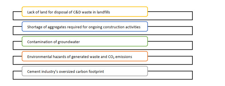
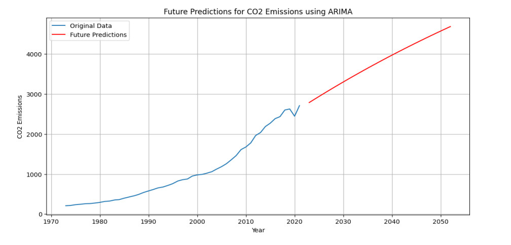
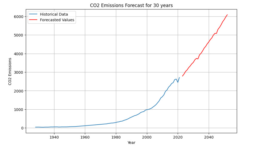
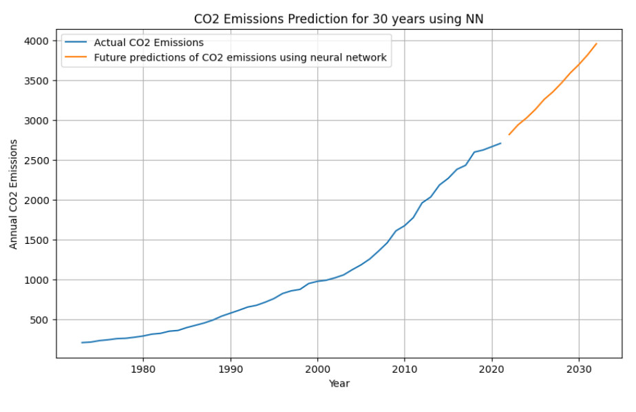
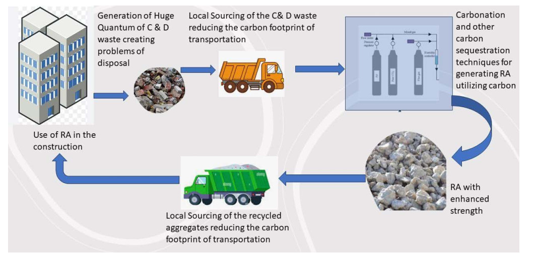
The cement industry's carbon emissions present a major global challenge, particularly the increase in atmospheric carbon dioxide (CO2) levels. The concrete industry is responsible for a significant portion of these emissions, accounting for approximately 5–9% of the total emissions. This underscores the urgent need for effective strategies to curb carbon emissions. In this work, we propose to use artificial intelligence (AI) to predict future emission trends by performing a detailed analysis of cement industry's CO2 emissions data. The AI predictive model shows a significant increase in overall carbon emissions from the cement sector which is attributed to population growth and increased demand for housing and infrastructure. To address this issue, we propose a framework that emphasizes on implementing carbon sequestration through reuse of construction and demolition (C & D) waste by using recycled aggregates. The paper proposes a framework addressing carbon sequestration through use of C & D waste. The framework is applied specifically to Maharashtra State in India to calculate the potential reduction in carbon emissions by construction industry resulting from recycled aggregates. The study reveals a projected saving of 24% in carbon emissions by adopting the suggested framework. The process and outcomes of the study aim to address the concerns of climate change through reduced carbon emissions in the construction industry promoting recycle and reuse of construction waste.
Citation: Sayali Sandbhor, Sayali Apte, Vaishnavi Dabir, Ketan Kotecha, Rajkumar Balasubramaniyan, Tanupriya Choudhury. AI-based carbon emission forecast and mitigation framework using recycled concrete aggregates: A sustainable approach for the construction industry[J]. AIMS Environmental Science, 2023, 10(6): 894-910. doi: 10.3934/environsci.2023048
The cement industry's carbon emissions present a major global challenge, particularly the increase in atmospheric carbon dioxide (CO2) levels. The concrete industry is responsible for a significant portion of these emissions, accounting for approximately 5–9% of the total emissions. This underscores the urgent need for effective strategies to curb carbon emissions. In this work, we propose to use artificial intelligence (AI) to predict future emission trends by performing a detailed analysis of cement industry's CO2 emissions data. The AI predictive model shows a significant increase in overall carbon emissions from the cement sector which is attributed to population growth and increased demand for housing and infrastructure. To address this issue, we propose a framework that emphasizes on implementing carbon sequestration through reuse of construction and demolition (C & D) waste by using recycled aggregates. The paper proposes a framework addressing carbon sequestration through use of C & D waste. The framework is applied specifically to Maharashtra State in India to calculate the potential reduction in carbon emissions by construction industry resulting from recycled aggregates. The study reveals a projected saving of 24% in carbon emissions by adopting the suggested framework. The process and outcomes of the study aim to address the concerns of climate change through reduced carbon emissions in the construction industry promoting recycle and reuse of construction waste.

| [1] |
Wang Y, Li X, Liu R (2022) The Capture and Transformation of Carbon Dioxide in Concrete: A Review. Symmetry 14: 2615. https://doi.org/10.3390/sym14122615 doi: 10.3390/sym14122615

|
| [2] |
Ali M B, Saidur R, Hossain M S (2011) A review on emission analysis in cement industries. Renew. Sustain. Energy Rev 15: 2252–2261. https://doi.org/10.1016/j.rser.2011.02.014 doi: 10.1016/j.rser.2011.02.014
|
| [3] |
Deja J, Uliasz-Bochenczyk A, Mokrzycki E (2010) CO2 emissions from the Polish cement industry. Int J Greenh Gas Control 4: 583–588. https://doi.org/10.1016/j.ijggc.2010.02.002 doi: 10.1016/j.ijggc.2010.02.002
|
| [4] |
Damineli B L, Kemeid F M, Aguiar P S, et al. (2010) Measuring the eco-efficiency of cement use. Cem Concr Compos 32: 555–562. https://doi.org/10.1016/j.cemconcomp.2010.07.009 doi: 10.1016/j.cemconcomp.2010.07.009
|
| [5] |
Nilimaa J, Zhaka V (2023) Material and Environmental Aspects of Concrete Flooring in Cold Climate. Constr Mat 3: 180-201. https://doi.org/10.3390/constrmater3020012 doi: 10.3390/constrmater3020012
|
| [6] | Scrivener, Karen, Vanderley M. John, and Ellis Bentz. Sustainable Concrete Construction. John Wiley & Sons, 2018. |
| [7] |
Nilimaa J, Gamil Y, Zhaka V (2023) Formwork Engineering for Sustainable Concrete Construction. Civi lEng 4: 1098-1120. https://doi.org/10.3390/civileng4040060 doi: 10.3390/civileng4040060
|
| [8] |
Tam V W Y, Butera A, Le K N, et al. (2021) CO2 concrete and its practical value utilizing living lab methodologies. Clean Eng Technol 3: 100131. https://doi.org/10.1016/j.clet.2021.100131 doi: 10.1016/j.clet.2021.100131
|
| [9] | Dhir, Ravindra K., Moray D (2012) Newlands, and Kenneth W. Paine. Concrete Sustainability. CRC Press. |
| [10] |
Nilimaa J (2023) Smart materials and technologies for sustainable concrete construction. Dev Built Environ 2023: 100177. https://doi.org/10.1016/j.dibe.2023.100177 doi: 10.1016/j.dibe.2023.100177
|
| [11] |
Feenstra R C, Inklaar R, Timmer M P (2015) The next generation of the Penn World Table. Am Econ Rev 105: 3150-3182. https://doi.org/10.1257/aer.20130954 doi: 10.1257/aer.20130954
|
| [12] | Max Roser (2013) Economic Growth Published online at OurWorldInData.org. Retrieved from: https://ourworldindata.org/economic-growth |
| [13] |
Blengini G A, Garbarino E (2010) Resources and waste management in Turin (Italy): the role of recycled aggregates in the sustainable supply mix. J Clean Prod 18: 1021-1030. https://doi.org/10.1016/j.jclepro.2010.01.027 doi: 10.1016/j.jclepro.2010.01.027
|
| [14] |
Liu Z, Meng W (2021) Fundamental understanding of carbonation curing and durability of carbonation-cured cement-based composites: A review. J CO2 Util 44: 101428. https://doi.org/10.1016/j.jcou.2020.101428 doi: 10.1016/j.jcou.2020.101428
|
| [15] | Zhang D, Ghouleh Z, Shao Y (2017) Review on carbonation curing of cement-based materials. J CO2 Util 21: 119-131. ttps://doi.org/10.1016/j.jcou.2017.07.003 |
| [16] | Jain M S. A mini review on generation, handling, and initiatives to tackle construction and demolition waste in India. Environ Technol Inno 22: 101490. https://doi.org/10.1016/j.eti.2021.101490 |
| [17] |
Tezeswi T P, MVN S K (2022) Implementing construction waste management in India: An extended theory of planned behaviour approach. Environ Technol Inno 27: 102401. https://doi.org/10.1016/j.eti.2022.102401 doi: 10.1016/j.eti.2022.102401
|
| [18] | Hertwich E G (2021) Increased carbon footprint of materials production driven by rise in investments. Nat Geosci 14: 151-155. |
| [19] |
Shi C, Li Y, Zhang J, et al. (2016) Performance enhancement of recycled concrete aggregate–a review. J Clean Prod 112: 466-472. https://doi.org/10.1016/j.jclepro.2015.08.057 doi: 10.1016/j.jclepro.2015.08.057
|
| [20] |
Younis K H, Pilakoutas K (2013) Strength prediction model and methods for improving recycled aggregate concrete. Constr Build Mater 49: 688-701. https://doi.org/10.1016/j.conbuildmat.2013.09.003 doi: 10.1016/j.conbuildmat.2013.09.003
|
| [21] |
Gomes M, de Brito J (2009) Structural concrete with incorporation of coarse recycled concrete and ceramic aggregates: durability performance. Mater Struct 42: 663-675. https://doi.org/10.1617/s11527-008-9411-9 doi: 10.1617/s11527-008-9411-9
|
| [22] |
Chen Y, Liu P, Yu Z (2018) Effects of environmental factors on concrete carbonation depth and compressive strength. Materials 11: 2167. https://doi.org/10.3390/ma11112167 doi: 10.3390/ma11112167
|
| [23] | He P, Shi C, Poon C S (2018) Methods for the assessment of carbon dioxide absorbed by cementitious materials[M]//Carbon Dioxide Sequestration in Cementitious Construction Materials. Woodhead Publishing, 2018: 103-126. https://doi.org/10.1016/B978-0-08-102444-7.00006-X |
| [24] |
Gomes H C, Reis E D, Azevedo R C, et al. (2023) Carbonation of Aggregates from Construction and Demolition Waste Applied to Concrete: A Review. Buildings 13: 1097. https://doi.org/10.3390/buildings13041097 doi: 10.3390/buildings13041097
|
| [25] |
Gomes R I, Farinha C B, Veiga R, et al. (2021) CO2 sequestration by construction and demolition waste aggregates and effect on mortars and concrete performance-An overview. Renew Sust Energ Rev 152: 111668. https://doi.org/10.1016/j.rser.2021.111668 doi: 10.1016/j.rser.2021.111668
|
| [26] |
Xiao J, Zhang H, Tang Y, et al. (2022) Fully utilizing carbonated recycled aggregates in concrete: Strength, drying shrinkage and carbon emissions analysis. J Clean Prod 377: 134520. https://doi.org/10.1016/j.jclepro.2022.134520 doi: 10.1016/j.jclepro.2022.134520
|
| [27] |
Wang T, Li K, Liu D, et al. (2022) Estimating the carbon emission of construction waste recycling using grey model and life cycle assessment: a case study of Shanghai. Int J Environ Res Public Health 19: 8507. https://doi.org/10.3390/ijerph19148507 doi: 10.3390/ijerph19148507
|
| [28] |
Liu H, Guo R, Tian J, et al. (2022) Quantifying the carbon reduction potential of recycling construction waste based on life cycle assessment: a case of Jiangsu province. Int J Environ Res Public Health 19: 12628. https://doi.org/10.3390/ijerph191912628 doi: 10.3390/ijerph191912628
|
Figures(15) / Tables(5)

Sayali Sandbhor, Sayali Apte, Vaishnavi Dabir, Ketan Kotecha, Rajkumar Balasubramaniyan, Tanupriya Choudhury. AI-based carbon emission forecast and mitigation framework using recycled concrete aggregates: A sustainable approach for the construction industry[J]. AIMS Environmental Science, 2023, 10(6): 894-910. doi: 10.3934/environsci.2023048


 DownLoad: