Reduction of greenhouse gas emissions in an imperfect production process under breakdown consideration

Bijoy Kumar Shaw; Isha Sangal; Biswajit Sarkar; Bijoy Kumar Shaw; Isha Sangal; Biswajit Sarkar

doi:10.3934/environsci.2022038

AIMS Environmental Science

2022, Volume 9, Issue 5: 658-691. doi: 10.3934/environsci.2022038

Previous Article Next Article

Research article Special Issues

Reduction of greenhouse gas emissions in an imperfect production process under breakdown consideration

1.
Department of Mathematics & Statistics, Banasthali Vidyapith, Banasthali, Rajasthan 304022, India
2.
Keranitola Shree Shree Mohanananda Vidyamandir (H.S.), Midnapore, Paschim Medinipur, West Bengal 721101, India
3.
Department of Industrial Engineering, Yonsei University, 50 Yonsei-ro, Sinchon-dong, Seodaemun-gu, Seoul 03722, South Korea
4.
Center for Transdisciplinary Research (CFTR), Saveetha Dental College, Saveetha Institute of Medical and Technical Sciences, Saveetha University, 162, Poonamallee High Road, Velappanchavadi, Chennai, Tamil Nadu 600077, India

Received: 07 May 2022 Revised: 27 June 2022 Accepted: 26 July 2022 Published: 09 October 2022

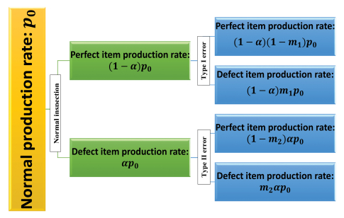
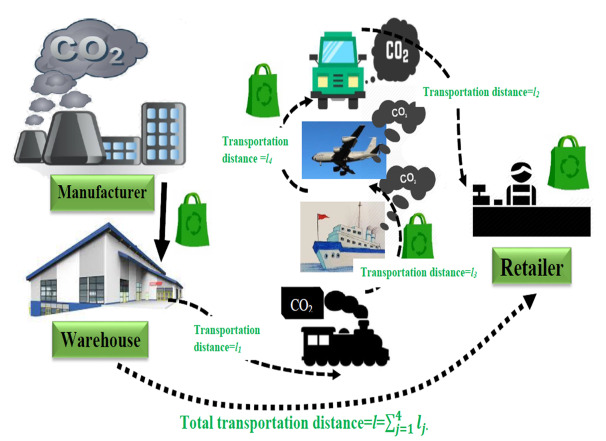
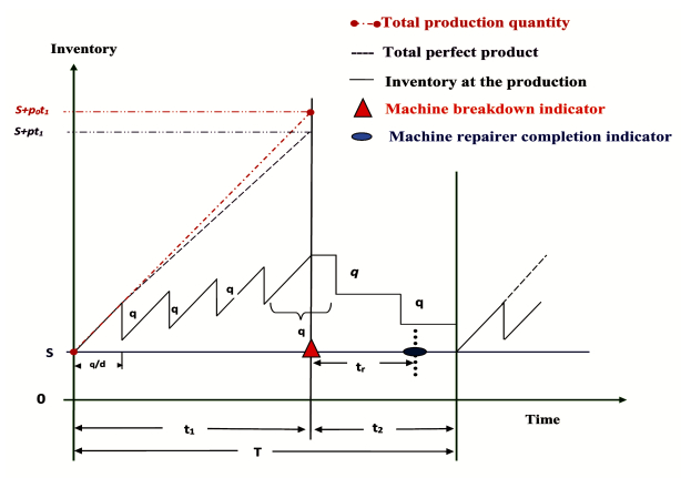
A long-run manufacturing system can experience machine breakdown at any time for various reasons such as unskilled labor or outdated machinery technology. In an integrated green inventory model, the produced green products cannot all be perfect throughout a cycle, particularly when machines malfunction. Therefore, an inspection policy is introduced to clean the production process from unusable defect products, the correctness of which depends on the discussion of the inspected errors. The perfect products detected via the inspection process are delivered to the retailer as well as the market. To transport green products, it is essential to control the capacity of the containers and the quantities of green products transported per batch. In this study, the greenhouse gas equivalence factor of CO$ _2 $ emissions is calculated for all green products' manufacturing and transportation mediums. These types of energies are used in the manufacturing process: electricity, natural gas, and coal. Whereas within transportation, four transportation modes are considered: railways, roadways, airways, and waterways. The retailer can agree to transport their inventories to the customers' house according to their requirement by requiring a third-party local agency via outsourcing criteria. The model solves the problem of CO$ _2 $ emissions through production and transportation within the machine breakdown.
- random machine breakdown,
- maintenance policy,
- transportation mode,
- energy consumption,
- greenhouse gas,
- carbon emissions
Citation: Bijoy Kumar Shaw, Isha Sangal, Biswajit Sarkar. Reduction of greenhouse gas emissions in an imperfect production process under breakdown consideration[J]. AIMS Environmental Science, 2022, 9(5): 658-691. doi: 10.3934/environsci.2022038

Related Papers:

Abstract

A long-run manufacturing system can experience machine breakdown at any time for various reasons such as unskilled labor or outdated machinery technology. In an integrated green inventory model, the produced green products cannot all be perfect throughout a cycle, particularly when machines malfunction. Therefore, an inspection policy is introduced to clean the production process from unusable defect products, the correctness of which depends on the discussion of the inspected errors. The perfect products detected via the inspection process are delivered to the retailer as well as the market. To transport green products, it is essential to control the capacity of the containers and the quantities of green products transported per batch. In this study, the greenhouse gas equivalence factor of CO$ _2 $ emissions is calculated for all green products' manufacturing and transportation mediums. These types of energies are used in the manufacturing process: electricity, natural gas, and coal. Whereas within transportation, four transportation modes are considered: railways, roadways, airways, and waterways. The retailer can agree to transport their inventories to the customers' house according to their requirement by requiring a third-party local agency via outsourcing criteria. The model solves the problem of CO$ _2 $ emissions through production and transportation within the machine breakdown.

References

[1]	Abisourour J, Hachkar M, Mounir B, et al. (2020) Methodology for integrated management system improvement: Combining costs deployment and value stream mapping. Int J Prod Res 58: 3667–3685. https://doi.org/10.1080/00207543.2019.1633482 doi: 10.1080/00207543.2019.1633482
[2]	Bai QG, Gong YM, Jin MZ, et. al (2019) Effects of carbon emission reduction on supply chain coordination with vendor-managed deteriorating product inventory. Int J Prod Econ 208: 83–99. http://doi.org/doi.org/10.1016/j.ijpe.2018.11.008. doi: 10.1016/j.ijpe.2018.11.008
[3]	Ben-Daya M, Hassini E, Bahroun Z (2019) Internet of things and supply chain management: A literature review. Int J Prod Res 57: 4719–4742. https://doi.org/10.1080/00207543.2017.1402140 doi: 10.1080/00207543.2017.1402140
[4]	Bhuniya S, Pareek P, Sarkar B, et al. (2021) A smart production process for the optimum energy consumption with maintenance policy under a supply chain managementy. Processes 9: 19. https://doi.org/10.3390/pr9010019 doi: 10.3390/pr9010019
[5]	Boulaksil Y, Grunow M, Fransoo JC (2011) Capacity flexibility allocation in an outsourced supply chain with reservation. Int J Prod Econ 129: 111–118. https://doi.org/10.1016/j.ijpe.2010.09.010 doi: 10.1016/j.ijpe.2010.09.010
[6]	Bouslah B, Gharbi A, Pellerin R, et al. (2013) Optimal production control policy in unreliable batch processing manufacturing systems with transportation delay. Int J Prod Res 51: 264–280. https://doi.org/10.1080/00207543.2012.676217 doi: 10.1080/00207543.2012.676217
[7]	Bortolini M, Faccio M, Gamberi M, et al. (2016) Multi-objective design of multi-modal fresh food distribution networks. Int J Logist Syst Manage 24: 155–177. https://doi.org/10.1504/IJLSM.2016.076470 doi: 10.1504/IJLSM.2016.076470
[8]	Cárdenas-Barrón LE, González-Velarde JL, Garza-Nuñeza D, et al. (2019) Heuristic algorithm based on reduce and optimize approach for a selective and periodic inventory routing problem in a waste vegetable oil collection environment. Int J Prod Econ 211: 44–59. http://doi.org/10.1016/j.ijpe.2019.01.026 doi: 10.1016/j.ijpe.2019.01.026
[9]	Cárdenas-Barrón LE, Shaikh AA, Tiwari S, et al. (2020) An EOQ inventory model with nonlinear stock dependent holding cost, nonlinear stock dependent demand and trade credit. Comput Ind Eng 139: 105557. https://doi.org/10.1016/j.cie.2018.12.004 doi: 10.1016/j.cie.2018.12.004
[10]	Cárdenas-Barrón LE, Treviño-Garza G (2014) An optimal solution to a three echelon supply chain network with multi-product and multi-period. Appl Math Model 38: 1911–1918. http://doi.org/10.1016/j.apm.2013.09.010 doi: 10.1016/j.apm.2013.09.010
[11]	Chan FTS, Wang ZX, Goswami A, et al. (2020) Multi-objective particle swarm optimisation based integrated production inventory routing planning for efficient perishable food logistics operations. Int J Prod Res 58: 5155–5174. https://doi.org/10.1080/00207543.2019.1701209 doi: 10.1080/00207543.2019.1701209
[12]	Chen YCK, Sackett PJ (2007) Return merchandize authorization stakeholders and customer requirements management—high-technology products. Int J Prod Res 45: 1595–1608. https://doi.org/10.1080/00207540600942508 doi: 10.1080/00207540600942508
[13]	Choi SB, Dey BK, Kim SJ, et al. (2022) Intelligent servicing strategy for an online-to-offline (O2O) supply chain under demand variability and controllable lead time. RAIRO-Oper Res 56: 1623–1653. https://doi.org/10.1051/ro/2022026 doi: 10.1051/ro/2022026
[14]	Elhedhli S, Merrick R (2012) Green supply chain network design to reduce carbon emissions. Transport Res D: Tr E 17: 370–379. http://doi.org/10.1016/j.trd.2012.02.002 doi: 10.1016/j.trd.2012.02.002
[15]	Faccio M, Persona A, Sgarbossa F, et al. (2011) Multi-stage supply network design in case of reverse flows: A closed-loop approach. Int J Oper Res 12: 157–191. https://doi.org/10.1504/IJOR.2011.042504 doi: 10.1504/IJOR.2011.042504
[16]	Faccio M, Gamberi M (2015) New city logistics paradigm: From the "Last Mile" to the "Last 50 Miles" sustainable distribution. Sustainability 7: 14873–14894. https://doi.org/10.3390/su71114873 doi: 10.3390/su71114873
[17]	Guchhait R, Sarkar B (2021) Economic and environmental assessment of an unreliable supply chain management. RAIRO-Oper Res 55: 3153–3170. https://doi.org/10.1051/ro/2021128 doi: 10.1051/ro/2021128
[18]	Ho KY, Su RK (2020) Insertion of new idle time for unrelated parallel machine scheduling with job splitting and machine breakdowns. Comput Ind Eng 147: 106630. https://doi.org/10.1016/j.cie.2020.106630 doi: 10.1016/j.cie.2020.106630
[19]	Hota SK, Ghosh SK, Sarkar B (2022) A solution to the transportation hazard problem in a supply chain with an unreliable manufacturer. AIMS Environ Sci 9: 354–380. http://doi.org/10.3934/environsci.2022023 doi: 10.3934/environsci.2022023
[20]	Jani MY, Betheja MR, Chaudhari U, et al. (2021) Optimal investment in preservation technology for variable demand under trade-credit and shortages. Mathematics 9: 1301. https://doi.org/10.3390/math9111301 doi: 10.3390/math9111301
[21]	Kaur J, Sidhu R, Awasthi A, et al. (2018) A dematel based approach for investigating barriers in green supply chain management in Canadian manufacturing firms. Int J Prod Res 56: 312–332. https://doi.org/10.1080/00207543.2017.1395522 doi: 10.1080/00207543.2017.1395522
[22]	Khan I, Sarkar B (2021) Transfer of risk in supply chain management with joint pricing and inventory decision considering shortages. Mathematics 9: 638. https://doi.org/10.3390/math9060638 doi: 10.3390/math9060638
[23]	Khan M, Hussain M, Cárdenas-Barrón LE, et al. (2017) Learning and screening errors in an EPQ inventory model for supply chains with stochastic lead time demands. Int J Prod Res 55: 4816–4832. https://doi.org/10.1080/00207543.2017.1310402 doi: 10.1080/00207543.2017.1310402
[24]	Kugele ASH, Ahmed W, Sarkar B (2022) Geometric programming solution of second degree difficulty for carbon ejection controlled reliable smart production system. RAIRO-Oper Res 56: 1013–1029. https://doi.org/10.1051/ro/2022028 doi: 10.1051/ro/2022028
[25]	Kumar S, Sigroha K, Kumar M, et al. (2022) Manufacturing/remanufacturing based supply chain management under advertisements and carbon emission process. RAIRO-Oper Res 56: 831–851. https://doi.org/10.1051/ro/2021189 doi: 10.1051/ro/2021189
[26]	Lee SD, Fu YC (2014) Joint production and delivery lot sizing for a make-to-order producer-buyer supply chain with transportation cost. Transp Res E: Log 66: 23–35. http://doi.org/10.1016/j.tre.2014.03.002 doi: 10.1016/j.tre.2014.03.002
[27]	Lee YH, Jeong CS, Moon C (2002) Advanced planning and scheduling with outsourcing in manufacturing supply chain. Comput Ind Eng 43: 351–374. https://doi.org/10.1016/S0360-8352(02)00079-7 doi: 10.1016/S0360-8352(02)00079-7
[28]	Majumder A, Sinha SS, Govindan K (2021) Prioritising risk mitigation strategies for environmentally sustainable clothing supply chains: Insights from selected organisational theories. Sustain Prod Consum 28: 543–555. https://doi.org/10.1016/j.spc.2021.06.021 doi: 10.1016/j.spc.2021.06.021
[29]	Muhammad I (2022) Carbon tax as the most appropriate carbon pricing mechanism for developing countries and strategies to design an effective policy. AIMS Environ Sci 9: 161–184. https://doi.org/10.3934/environsci.2022012 doi: 10.3934/environsci.2022012
[30]	Mittal M, Pareek S, Agarwal R (2015) EOQ estimation for imperfect quality items using association rule mining with clustering. Decis Sci Lett 4: 497–508. http://doi.org/10.5267/j.dsl.2015.5.008 doi: 10.5267/j.dsl.2015.5.008
[31]	Mittal M, Sarkar B (2022) Stochastic behavior of exchange rate on an international supply chain under random energy price. Math Comput Simulat. In press. https://doi.org/10.1016/j.matcom.2022.09.007
[32]	Moon I, Yun WY, Sarkar B (2022) Effects of variable setup cost, reliability, and production costs under controlled carbon emissions in a reliable production system. Eur J Ind Eng 16: 371–397.
[33]	Nguyen L, Moseson AJ, Spatari S, et al. (2018) Effects of composition and transportation logistics on environmental, energy and cost metrics for the production of alternative cementitious binders. J Clean Prod 185: 628–645. http://doi.org/10.1016/j.jclepro.2018.02.247 doi: 10.1016/j.jclepro.2018.02.247
[34]	Sana SS, Chaudhuri K (2010) An EMQ model in an imperfect production process. Int J Syst Sci 41: 635–646. http://doi.org/10.1080/00207720903144495 doi: 10.1080/00207720903144495
[35]	Sarkar A, Guchhait R, Sarkar B (2022) Application of the artificial neural network with multithreading within an inventory model under uncertainty and inflation. Int J Fuzzy Syst 24: 2318–2332. https://doi.org/10.1007/s40815-022-01276-1 doi: 10.1007/s40815-022-01276-1
[36]	Sarkar B, Bhuniya B (2022) A sustainable flexible manufacturing–remanufacturing model with improved service and green investment under variable demand. Expert Syst Appl 202: 117154. https://doi.org/10.1016/j.eswa.2022.117154 doi: 10.1016/j.eswa.2022.117154
[37]	Sarkar B, Dey BK, Sarkar M, et al. (2022) A smart production system with an autonomation technology and dual channel retailing. Comput Ind Eng 173: 108607. https://doi.org/10.1016/j.cie.2022.108607 doi: 10.1016/j.cie.2022.108607
[38]	Sarkar B, Joo J, Kim Y, et al. (2022) Controlling defective items in a complex multi-phase manufacturing system. RAIRO-Oper Res 56: 871–889. https://doi.org/10.1051/ro/2022019 doi: 10.1051/ro/2022019
[39]	Sarkar B, Kar S, Basu K, et al. (2022) A sustainable managerial decision-making problem for a substitutable product in a dual-channel under carbon tax policy. Comput Ind Eng 172: 108635. http://doi.org/10.1016/j.cie.2022.108635 doi: 10.1016/j.cie.2022.108635
[40]	Sarkar B, Saren S (2016) Product inspection policy for an imperfect production system with inspection errors and warranty cost. Eur J Oper Res 248: 263–271. http://doi.org/10.1016/j.ejor.2015.06.021 doi: 10.1016/j.ejor.2015.06.021
[41]	Sarkar B, Takeyeva D, Guchhait R, et al. (2022) Optimized radio-frequency identification system for different warehouse shapes. Know-Based Syst. In press. https://doi.org/10.1016/j.knosys.2022.109811
[42]	Shekarian E, Marandi A, Majava J (2021) Dual-channel remanufacturing closed-loop supply chains under carbon footprint and collection competition. Sustain Prod Consum 28: 1050–1075. https://doi.org/10.1016/j.spc.2021.06.028 doi: 10.1016/j.spc.2021.06.028
[43]	Tayyab M, Habib MS, Jajja MSS, et al. (2022) Economic assessment of a serial production system with random imperfection and shortages: A step towards sustainability. Comput Ind Eng 171: 108398. https://doi.org/10.1016/j.cie.2022.108398 doi: 10.1016/j.cie.2022.108398
[44]	Taleizadeh AA, Cárdenas-Barrón LE, Sohani R (2019) Coordinating the supplier-retailer supply chain under noise effect with bundling and inventory strategies. J Ind Manag Optim 15: 1701–1727. http://doi.org/10.3934/jimo.2018118 doi: 10.3934/jimo.2018118
[45]	Tseng SC, Hung SW (2014) A strategic decision-making model considering the social costs of carbon dioxide emissions for sustainable supply chain management. J Environ Manage 133: 315–322. http://doi.org/10.1016/j.jenvman.2013.11.023 doi: 10.1016/j.jenvman.2013.11.023
[46]	Ullah M, Asghar I, Zahid M, et al. (2021) Ramification of remanufacturing in a sustainable three-echelon closed-loop supply chain management for returnable products. J Clean Prod 290: 125609. https://doi.org/10.1016/j.jclepro.2020.125609 doi: 10.1016/j.jclepro.2020.125609
[47]	Wee HM, Daryanto Y (2020) Imperfect quality item inventory models considering carbon emissions, In: Shah N, Mittal M (Eds.), Optimization and inventory management, Singapore: Springer, 137–159. http://doi.org/10.1007/978-981-13-9698-4_8
[48]	Zhu ZG, Chu F, Dolgui A, et al. (2017) Recent advances and opportunities in sustainable food supply chain: A model-oriented review. Int J Prod Res 56: 5700–5722. https://doi.org/10.1080/00207543.2018.1425014 doi: 10.1080/00207543.2018.1425014

Reader Comments

your name:*

Email:*
© 2022 the Author(s), licensee AIMS Press. This is an open access article distributed under the terms of the Creative Commons Attribution License (http://creativecommons.org/licenses/by/4.0)