The definition of environmental indexes is one of the most widely used methods and methodologies for the study of exposure to polluting agents, and it is a highly helpful instrument for describing the quality of the environment in a simple and straightforward manner. In this study, index models were presented and described that can be used in evaluating the contamination, pollution and health risks of environmental micro (MPs) and nanoplastics (NPs) to ecosystems and humans. Index models such as plastic contamination factors (pCf) and pollution load index (pPLI), plastic- bioconcentration or accumulation factors (pBCf or pBAf), plastic-biota-sediment accumulation factor (pBSAf), biota accumulation load index (BALI), polymer risks indices (pRi), polymer ecological risks index (pERI) while plastic estimated daily intake (pEDI) and plastic carcinogenic risks (pCR) were described for oral, dermal and inhalation pathways. All index modeled were further described based on polymer types of MPs/NPs. The final value is represented by a quantity that measures a weighted combination of sub-indices and defined by an appropriate mathematical function. The central concept is to present an indicator that can describe, in a clear and concise manner, the level of MPs/NPs in the environment, thereby indicating where it would be necessary to intervene and where it would not in order to improve overall environmental conditions.
Citation: Ebere Enyoh Christian, Qingyue Wang, Wirnkor Verla Andrew, Chowdhury Tanzin. Index models for ecological and health risks assessment of environmental micro-and nano-sized plastics[J]. AIMS Environmental Science, 2022, 9(1): 51-65. doi: 10.3934/environsci.2022004
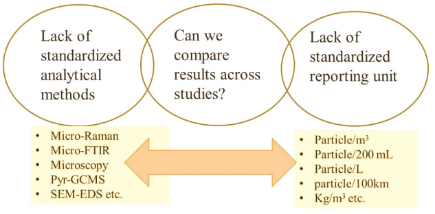
The definition of environmental indexes is one of the most widely used methods and methodologies for the study of exposure to polluting agents, and it is a highly helpful instrument for describing the quality of the environment in a simple and straightforward manner. In this study, index models were presented and described that can be used in evaluating the contamination, pollution and health risks of environmental micro (MPs) and nanoplastics (NPs) to ecosystems and humans. Index models such as plastic contamination factors (pCf) and pollution load index (pPLI), plastic- bioconcentration or accumulation factors (pBCf or pBAf), plastic-biota-sediment accumulation factor (pBSAf), biota accumulation load index (BALI), polymer risks indices (pRi), polymer ecological risks index (pERI) while plastic estimated daily intake (pEDI) and plastic carcinogenic risks (pCR) were described for oral, dermal and inhalation pathways. All index modeled were further described based on polymer types of MPs/NPs. The final value is represented by a quantity that measures a weighted combination of sub-indices and defined by an appropriate mathematical function. The central concept is to present an indicator that can describe, in a clear and concise manner, the level of MPs/NPs in the environment, thereby indicating where it would be necessary to intervene and where it would not in order to improve overall environmental conditions.

| [1] |
Duis K, Coors A (2016) Microplastics in the aquatic and terrestrial environment: sources (with a specific focus on personal care products), fate and effects. Environ Sci Eur 28: 2–13. https://doi.org/10.1186/s12302-015-0069-y doi: 10.1186/s12302-015-0069-y

|
| [2] |
Verla AW, Enyoh CE, Verla EN, et al. (2019) Microplastic-Toxic Chemical Interaction: a Review Study on Quantified Levels, Mechanism and Implications. Spr Nature Appl Sci 1: 1400–1441. https://doi.org/10.1007/s42452-019-1352-0 doi: 10.1007/s42452-019-1352-0
|
| [3] |
Haegerbaeumer A, Mueller MT, Fueser H, et al. (2019) Impacts of Micro- and Nano-Sized Plastic Particles on Benthic Invertebrates: A Literature Review and Gap Analysis. Front Environ Sci 7: 17. https://10.3389/fenvs.2019.00017 doi: 10.3389/fenvs.2019.00017
|
| [4] |
Wang Q, Enyoh CE, Chowdhury T, et al. (2020). Analytical Techniques, Occurrence and Health Effects of Micro and Nano Plastics Deposited in Street Dust. Intl J Environ Anal Chem 28: 1.16. https://doi.org/10.1080/03067319.2020.1811262 doi: 10.1080/03067319.2020.1811262
|
| [5] | Qiao R, Sheng C, Lu Y, et al. (2019) Microplastics induce intestinal inflammation, oxidative stress, and disorders of metabolome and microbiome in zebrafish. Sci Total Environ 662: 246–253. |
| [6] |
Yee MS, Hii LW, Looi CK, et al. (2021) Impact of Microplastics and Nanoplastics on Human Health. Nanomaterials 11: 496–510. https://doi.org/10.3390/nano11020496 doi: 10.3390/nano11020496
|
| [7] | Ziajahromi S, Kumar A, Neale PA, et al. (2017) Impact of microplastic beads and fibers on waterflea (Ceriodaphnia dubia) survival, growth, and reproduction: implications of single and mixture exposures. Environ Sci Technol 51: 13397–13406. |
| [8] | Zimmermann L, Dierkes G, Ternes TA, et al. (2019) Benchmarking the in vitro toxicity and chemical composition of plastic consumer products. Environ Sci Technol 53: 11467–11477.9 |
| [9] | Rochman CM, Brookson C, Bikker J, et al. (2019) Rethinking microplastics as a diverse contaminant suite. Environ Toxicol Chem 38: 703–711. |
| [10] |
Enyoh CE, Shafea L, Verla AW, et al. (2020). Microplastics Exposure Routes and Toxicity Studies to Ecosystems: An Overview. Environ Analy Health Toxic 35: 1–10. https://doi.org/10.5620/eaht.e2020004. doi: 10.5620/eaht.e2020004
|
| [11] | Gray AD, Weinstein JE (2017) Size- and shape-dependent effects of microplastic particles on adult daggerblade grass shrimp (Palaemonetes pugio). Environ Toxicol Chem36: 3074–3080. |
| [12] | Botterell ZLR, Beaumont N, Dorrington T, et. al. (2019) Bioavailability and effects of microplastics on marine zooplankton: a review. Environ Pollut 245: 98–110. |
| [13] | Hall NM, Berry KLE, Rintoul L, et al. (2015) Microplastic ingestion by scleractinian corals. Mar Biol 162: 725–732. |
| [14] | Ott WR (1978) Environmental Indices: Theory and Practice, Ann Arbor Science Publ. Inc., Michigan. |
| [15] | Malkina-Pykh IG, Pyk YA (1999) Environmental indices design and integrated modelling: theory and application. Eco Sus Dev12: 123–132. |
| [16] |
Smith L, Turrell WR (2021) Monitoring Plastic Beach Litter by Number or by Weight: The Implications of Fragmentation. Front Mar Sci 8: 702570. https://10.3389/fmars.2021.702570 doi: 10.3389/fmars.2021.702570
|
| [17] |
Enyoh CE, Wirnkor VA, Ngozi VE, et al. (2019). Macrodebris and microplastics pollution in Nigeria: first report on abundance, distribution and composition. Environ Analy Health Toxic 34: e2019012. https://doi.org/10.5620/eaht.e2019012 doi: 10.5620/eaht.e2019012
|
| [18] | Matlack AS. Introduction to green chemistry. New York: Marcel Decker Inc; 2001. National Environmental Protection Agency of China (NEPAC) (2014) Technical Guidance for Risk Assessment to Contaminated Sites; HJ25.3-2014; NEPAC: Beijing, China. Plewig G, Kligman AM. Acne and Rosacea. 3rd edition. Berlin, Heidelberg: Springer; 2000. |
| [19] | Araújo PHH, Sayer C, Poco JGR, et al. (2002) Techniques for reducing residual monomer content in polymers: a review. Polym Eng Sci 42: 1442–1468. |
| [20] |
Lithner D, Larsson A, Dave G (2011) Environmental and health hazard ranking and assessment of plastic polymers based on chemical composition. Sci Total Environ 409: 3309–3324. https://doi.org/10.1016/j.scitotenv.2011.04.038 doi: 10.1016/j.scitotenv.2011.04.038
|
| [21] | Kabir EAHM, Masahiko S, Tsuyoshi I, et al. (2021) Assessing small-scale freshwater microplastics pollution, land-use, source-to-sink conduits, and pollution risks: Perspectives from Japanese rivers polluted with microplastics. Sci Total Environ 768: 144655. |
| [22] | Enyoh CE, Verla AW, Rakib MRJ (2021). Application of Index Models for Assessing Freshwater Microplastics Pollution, World News Nat Sci 38: 37–48. |
| [23] |
Ibeto CN, Enyoh CE, Ofomatah AC, et al. (2021) Microplastics pollution indices of bottled water from South Eastern Nigeria. Intl J Environ Anal Chem 38: 27–38. DOI: 10.1080/03067319.2021.1982926 doi: 10.1080/03067319.2021.1982926
|
| [24] |
Catarino AI, Valeria M, William GS, et al. (2018) Low levels of microplastics (MP) in wild mussels indicate that MP ingestion by humans is minimal compared to exposure via household fibres fallout during a meal. Environ Poll 237: 675–684. https://doi.org/10.1016/j.envpol.2018.02.069 doi: 10.1016/j.envpol.2018.02.069
|
| [25] | Enyoh CE, Verla AW, Verla EN (2019) Uptake of microplastics by plant: a reason to worry or to be happy? World Sci News 131: 256–267 |
| [26] | USEPA (2011) Exposure Factors Handbook 2011 Edition (Final); Office of Emergency and Remedial Response: Washington, DC, USA. |
| [27] | Jo HY, Yu DS, Oh CH (2007) Quantitative research on skin pore widening using a stereoimage optical topometer and Sebutape. Skin Res Technol 13: 162–168. |
| [28] | Saedi N, Petrell K, Arndt K, et al. (2013) Evaluating facial pores and skin texture after low-energy nonablative fractional 1440-nm laser treatments. J Am Acad Dermatol 68: 113–118. |
| [29] | USEPA (2002) Supplemental Guidance for Developing Soil Screening Levels for Superfund Sites; Office of Emergency and Remedial Response: Washington, DC, USA. |
| [30] |
Valderrama C, Gamisans X, de las Heras X, et al. (2008) Sorption kinetics of polycyclic aromatic hydrocarbons removal using granular activated carbon: intraparticle diffusion coefficients. J Hazard Mater 157: 386–396. https://doi.org/10.1016/j.jhazmat.2007.12.119. doi: 10.1016/j.jhazmat.2007.12.119
|
| [31] | Wilke CR, Chang P (1955) Correlation of diffusion coefficients in dilute solutions. AIChE J 1: 264–270 |
| [32] | Gasperi J, Wright SL, Dris R, et al. (2018) Microplastics in air: are we breathing it in? Curr Opin Environ Sci Health 1: 1–5 |
| [33] |
Enyoh CE, Verla AW, Verla EN, et al. (2019). Airborne Microplastics: a Review Study on Method for Analysis, Occurrence, Movement and Risks. Environ Monitor Assess 191: 1–11. https://doi.org/10.1007/s10661-019-7842-0. doi: 10.1007/s10661-019-7842-0
|
| [34] | WHO (1997) Determination of airborne fibre number concentrations: a recommended method, by phase contrast optical microscopy (membrane filter method). https://apps.who.int/iris/handle/10665/41904 Assessed 28/08/2021. |
| [35] | USEPA (1992) Health Assessment Summary Tables. Annual FY-92. Prepared by the Office of Health and Environmental Assessment, Environmental Criteria and Assessment Office, Cincinnati, OH, for the Office of Emergency and Remedial Response, Washington, DC. |
| [36] | USEPA (1997). Toxics Release Inventory Relative Risk-Based Environmental Indicators: Interim Toxicity Weighting Summary Document. Pp. 1–252. https://www.epa.gov/sites/production/files/2014-03/documents/toxwght97.pdf |

Figures(2) / Tables(1)

Ebere Enyoh Christian, Qingyue Wang, Wirnkor Verla Andrew, Chowdhury Tanzin. Index models for ecological and health risks assessment of environmental micro-and nano-sized plastics[J]. AIMS Environmental Science, 2022, 9(1): 51-65. doi: 10.3934/environsci.2022004


 DownLoad: