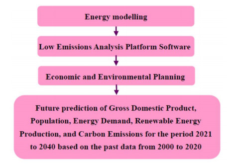
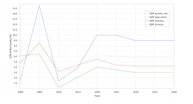
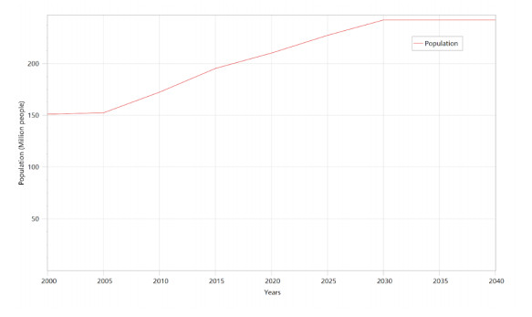
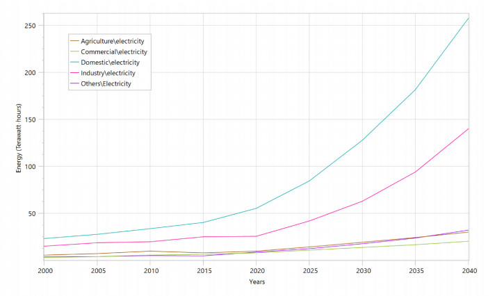
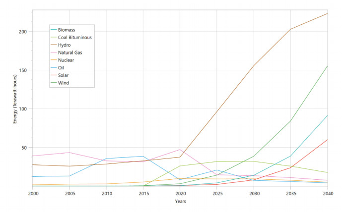
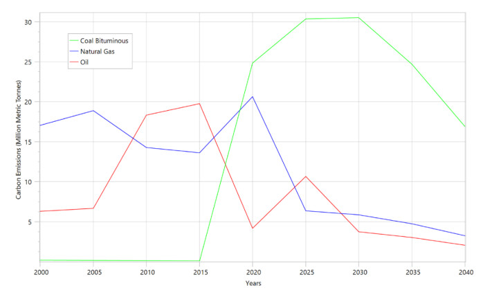
The Government of Pakistan has established clean energy transition goals in the national Alternative and Renewable Energy (ARE) Policy. The goal of this policy is to increase the 30% capacity of green energy in total energy mix by 2030. In this regard, the aim of this study is to develop a de-carbonization plan for achieving net zero emissions through the deployment of a green energy system for the period 2021 to 2040 by incorporating the ARE policy targets. The Low Emissions Analysis Platform (LEAP®) software is used for finding the unidirectional causality among gross domestic product, population within the country, energy demand, renewable energy production and CO2 emissions for Pakistan. The results revealed that energy production of 564.16 TWh is enough to meet the energy demand of 480.10 TWh with CO2 emissions of 22.19 million metric tons, having a population of 242.1 million people and GDP growth rate of 5.8%, in the year 2040 in Pakistan. The share of green energy production is 535.07 TWh, which can be utilized fully for meeting energy demand in the country, and almost zero emissions will produce till 2040. CO2 emissions produced by burning natural gas were 20.64 million metric tons in 2020, which then reduced to 3.25 million metric tons in 2040. CO2 emissions produced by burning furnace oil are also reduced from 4.19 million metric tons in 2020 to 2.06 million metric tons in 2040. CO2 emissions produced by burning coal were 24.85 million metric tons in 2020, which then reduced to 16.88 million metric tons in 2040. Energy demand is directly related to the population and GDP of the country, while renewable utilization is inversely proportional to carbon emissions. The declining trend of carbon emissions in Pakistan would help to achieve net zero emissions targets by mid-century. This technique would bring prosperity in the development of a clean, green and sustainable environment.
Citation: Muhammad Amir Raza, M. M. Aman, Abdul Ghani Abro, Muhammad Shahid, Darakhshan Ara, Tufail Ahmed Waseer, Mohsin Ali Tunio, Nadeem Ahmed Tunio, Shakir Ali Soomro, Touqeer Ahmed Jumani. The role of techno-economic factors for net zero carbon emissions in Pakistan[J]. AIMS Energy, 2023, 11(2): 239-255. doi: 10.3934/energy.2023013
The Government of Pakistan has established clean energy transition goals in the national Alternative and Renewable Energy (ARE) Policy. The goal of this policy is to increase the 30% capacity of green energy in total energy mix by 2030. In this regard, the aim of this study is to develop a de-carbonization plan for achieving net zero emissions through the deployment of a green energy system for the period 2021 to 2040 by incorporating the ARE policy targets. The Low Emissions Analysis Platform (LEAP®) software is used for finding the unidirectional causality among gross domestic product, population within the country, energy demand, renewable energy production and CO2 emissions for Pakistan. The results revealed that energy production of 564.16 TWh is enough to meet the energy demand of 480.10 TWh with CO2 emissions of 22.19 million metric tons, having a population of 242.1 million people and GDP growth rate of 5.8%, in the year 2040 in Pakistan. The share of green energy production is 535.07 TWh, which can be utilized fully for meeting energy demand in the country, and almost zero emissions will produce till 2040. CO2 emissions produced by burning natural gas were 20.64 million metric tons in 2020, which then reduced to 3.25 million metric tons in 2040. CO2 emissions produced by burning furnace oil are also reduced from 4.19 million metric tons in 2020 to 2.06 million metric tons in 2040. CO2 emissions produced by burning coal were 24.85 million metric tons in 2020, which then reduced to 16.88 million metric tons in 2040. Energy demand is directly related to the population and GDP of the country, while renewable utilization is inversely proportional to carbon emissions. The declining trend of carbon emissions in Pakistan would help to achieve net zero emissions targets by mid-century. This technique would bring prosperity in the development of a clean, green and sustainable environment.

| [1] |
Bennich T, Weitz N, Carlsen H (2020) Deciphering the scientific literature on SDG interactions: A review and reading guide. Sci Total Environ 728: 138405. https://doi.org/10.1016/j.scitotenv.2020.138405 doi: 10.1016/j.scitotenv.2020.138405

|
| [2] |
Breuer A, Janetschek H, Malerba D (2019) Translating sustainable development goal (SDG) interdependencies into policy advice. Sustainability 11: 2092. https://doi.org/10.3390/su11072092 doi: 10.3390/su11072092
|
| [3] |
Leal Filho W, Azeiteiro U, Alves F, et al. (2018) Reinvigorating the sustainable development research agenda: the role of the sustainable development goals (SDG). Int J Sustainable Dev World Ecol 25: 131–142. https://doi.org/10.1080/13504509.2017.1342103 doi: 10.1080/13504509.2017.1342103
|
| [4] |
Campbell BM, Hansen J, Rioux J, et al. (2018) Urgent action to combat climate change and its impacts (SDG 13): Transforming agriculture and food systems. Curr Opin Environ Sustainability 34: 13–20. https://doi.org/10.1016/j.cosust.2018.06.005 doi: 10.1016/j.cosust.2018.06.005
|
| [5] |
Schmidt-Traub G, Kroll C, Teksoz K, et al. (2017) National baselines for the sustainable development goals assessed in the SDG index and dashboards. Nat Geosci 10: 547–555. https://doi.org/10.1038/NGEO2985 doi: 10.1038/NGEO2985
|
| [6] |
Diaz-Sarachaga JM, Jato-Espino D, Castro-Fresno D (2018) Is the Sustainable Development Goals (SDG) index an adequate framework to measure the progress of the 2030 Agenda? Sustainable Dev 26: 663–671. https://doi.org/10.1002/sd.1735 doi: 10.1002/sd.1735
|
| [7] |
Shahbaz M, Sharma R, Sinha A, et al. (2021) Analyzing nonlinear impact of economic growth drivers on CO2 emissions: Designing an SDG framework for India. Energy Pol 148: 111965. https://doi.org/10.1016/j.enpol.2020.111965 doi: 10.1016/j.enpol.2020.111965
|
| [8] |
Raza MA, Khatri KL, Rafique K, et al. (2021) Harnessing electrical power from hybrid biomass-solid waste energy resources for microgrids in underdeveloped and developing countries. Eng Technol Appl Sci Res 11: 7257–7261. https://doi.org/10.48084/etasr.4177 doi: 10.48084/etasr.4177
|
| [9] |
Shahbaz MS, Kazi AG, Othman B, et al. (2019) Identification, assessment and mitigation of environment side risks for Malaysian manufacturing. Eng Technol Appl Sci Res 9: 3851–3857. https://doi.org/10.48084/etasr.2529 doi: 10.48084/etasr.2529
|
| [10] |
Sinha A, Sengupta T, Kalugina O, et al. (2020) Does distribution of energy innovation impact distribution of income: A quantile-based SDG modeling approach. Technol Forecasting Social Change 160: 120224. https://doi.org/10.1016/j.techfore.2020.120224 doi: 10.1016/j.techfore.2020.120224
|
| [11] |
Awan A, Bilgili F (2022) Energy poverty trends and determinants in Pakistan: Empirical evidence from eight waves of HIES 1998–2019. Renewable Sustainable Energy Rev 158: 112157. https://doi.org/10.1016/j.rser.2022.112157 doi: 10.1016/j.rser.2022.112157
|
| [12] |
Hassan M, Khan Afridi M, Irfan Khan M (2019) Energy policies and environmental security: A multi-criteria analysis of energy policies of Pakistan. Int J Green Energy 16: 510–519. https://doi.org/10.1080/15435075.2019.1593177 doi: 10.1080/15435075.2019.1593177
|
| [13] |
Raza MA, Khatri KL, Haque MIU, et al. (2022) Holistic and scientific approach to the development of sustainable energy policy framework for energy security in Pakistan. Energy Rep 8: 4282–4302. https://doi.org/10.1016/j.egyr.2022.03.044 doi: 10.1016/j.egyr.2022.03.044
|
| [14] |
Raza MA, Khatri KL, Memon MA, et al. (2022) Exploitation of Thar coal field for power generation in Pakistan: A way forward to sustainable energy future. Energy Explor Exploit. 40: 1173–1196. https://doi.org/10.1177/01445987221082190 doi: 10.1177/01445987221082190
|
| [15] |
Raza MA, Khatri KL, Israr A, et al. (2022) Energy demand and production forecasting in Pakistan. Energy Strat Rev 39: 100788. https://doi.org/10.1016/j.esr.2021.100788 doi: 10.1016/j.esr.2021.100788
|
| [16] |
Raza MA, Khatri KL, Hussain A (2022) Transition from fossilized to defossilized energy system in Pakistan. Renewable Energy 190: 19–29. https://doi.org/10.1016/j.renene.2022.03.059 doi: 10.1016/j.renene.2022.03.059
|
| [17] |
Raza MA, Khatri KL, Akbar S, et al. (2021) Towards improving technical performance of a 747 MW thermal power plant. Quaid-E-Awam Uni Res J Eng Sci Technol Nawabshah 19: 104–111. https://doi.org/10.52584/QRJ.1901.15 doi: 10.52584/QRJ.1901.15
|
| [18] |
Abbasi SA, Harijan K, Khan MWA, et al. (2021) Long-term optimal power generation pathways for Pakistan. Energy Sci Eng 9: 2252–2267. https://doi.org/10.1002/ese3.981 doi: 10.1002/ese3.981
|
| [19] |
Palconit EV, Villanueva JR, Enano N, et al. (2021) Resource assessment of tidal stream power in Pakiputan Strait, Davao Gulf, Philippines. Eng Technol Appl Sci Res 11: 7233–7239. https://doi.org/10.48084/etasr.3853 doi: 10.48084/etasr.3853
|
| [20] |
Pao H-T, Tsai C-M (2011) Modeling and forecasting the CO2 emissions, energy consumption, and economic growth in Brazil. Energy 36: 2450–2458. https://doi.org/10.1016/j.energy.2011.01.032 doi: 10.1016/j.energy.2011.01.032
|
| [21] |
Saboori B, Sulaiman J (2013) Environmental degradation, economic growth and energy consumption: Evidence of the environmental Kuznets curve in Malaysia. Energy Pol 60: 892–905. https://doi.org/10.1016/j.enpol.2013.05.099 doi: 10.1016/j.enpol.2013.05.099
|
| [22] |
Pao H-T, Yu H-C, Yang Y-H (2011) Modeling the CO2 emissions, energy use, and economic growth in Russia. Energy 36: 5094–5100. https://doi.org/10.1016/j.energy.2011.06.004 doi: 10.1016/j.energy.2011.06.004
|
| [23] |
Nasir M, Rehman FU (2011) Environmental Kuznets curve for carbon emissions in Pakistan: An empirical investigation. Energy Policy 39: 1857–1864. https://doi.org/10.1016/j.enpol.2011.01.025 doi: 10.1016/j.enpol.2011.01.025
|
| [24] |
Wang SS, Zhou DQ, Zhou P, et al. (2011) CO2 emissions, energy consumption and economic growth in China: A panel data analysis. Energy Policy 39: 4870–4875. https://doi.org/10.1016/j.enpol.2011.06.032 doi: 10.1016/j.enpol.2011.06.032
|
| [25] |
Hao Y, Liu Y, Weng J-H, et al. (2016) Does the Environmental Kuznets Curve for coal consumption in China exist? New evidence from spatial econometric analysis. Energy 114: 1214–1223. https://doi.org/10.1016/j.energy.2016.08.075 doi: 10.1016/j.energy.2016.08.075
|
| [26] |
Saboori B, Sulaiman J, Mohd S (2012) Economic growth and CO2 emissions in Malaysia: A cointegration analysis of the environmental Kuznets curve. Energy Policy 51: 184–191. https://doi.org/10.1016/j.enpol.2012.08.065 doi: 10.1016/j.enpol.2012.08.065
|
| [27] |
Ozturk I, Acaravci A (2010) CO2 emissions, energy consumption and economic growth in Turkey. Renewable Sustainable Energy Rev 14: 3220–3225. https://doi.org/10.1016/j.rser.2010.07.005 doi: 10.1016/j.rser.2010.07.005
|
| [28] |
Ozturk I, Acaravci A (2013) The long-run and causal analysis of energy, growth, openness and financial development on carbon emissions in Turkey. Energy Econo 36: 262–267. https://doi.org/10.1016/j.eneco.2012.08.025 doi: 10.1016/j.eneco.2012.08.025
|
| [29] |
Apergis N, Payne JE (2010) The emissions, energy consumption, and growth nexus: evidence from the commonwealth of independent states. Energy Policy 38: 650–655. https://doi.org/10.1016/j.enpol.2009.08.029 doi: 10.1016/j.enpol.2009.08.029
|
| [30] |
Jaunky VC (2011) The CO2 emissions-income nexus: Evidence from rich countries. Energy Policy 39: 1228–1240. https://doi.org/10.1016/j.enpol.2010.11.050 doi: 10.1016/j.enpol.2010.11.050
|
| [31] |
Acaravci A, Ozturk I (2010) On the relationship between energy consumption, CO2 emissions and economic growth in Europe. Energy 35: 5412–5420. https://doi.org/10.1016/j.energy.2010.07.009 doi: 10.1016/j.energy.2010.07.009
|
| [32] |
Saboori B, Sulaiman J (2013) CO2 emissions, energy consumption and economic growth in Association of Southeast Asian Nations (ASEAN) countries: A cointegration approach. Energy 55: 813–822. https://doi.org/10.1016/j.energy.2013.04.038 doi: 10.1016/j.energy.2013.04.038
|
| [33] |
Zaman K, Shahbaz M, Loganathan N, et al. (2016) Tourism development, energy consumption and Environmental Kuznets Curve: Trivariate analysis in the panel of developed and developing countries. Tourism Manage 54: 275–283. https://doi.org/10.1016/j.tourman.2015.12.001 doi: 10.1016/j.tourman.2015.12.001
|
| [34] |
Shahbaz M, Mutascu M, Azim P (2013) Environmental Kuznets curve in Romania and the role of energy consumption. Renewable Sustainable Energy Rev 18: 165–173. https://doi.org/10.1016/j.rser.2012.10.012 doi: 10.1016/j.rser.2012.10.012
|
| [35] |
Tiwari AK, Shahbaz M, Hye QMA (2013) The environmental Kuznets curve and the role of coal consumption in India: cointegration and causality analysis in an open economy. Renewable Sustainable Energy Rev 18: 519–527. https://doi.org/10.1016/j.rser.2012.10.031 doi: 10.1016/j.rser.2012.10.031
|
| [36] |
Yavuz NÇ (2014) CO2 emission, energy consumption, and economic growth for Turkey: evidence from a cointegration test with a structural break. Energy Sources, Part B: Economics, Planning, Policy 9: 229–235. https://doi.org/10.1080/15567249.2011.567222 doi: 10.1080/15567249.2011.567222
|
| [37] |
Akbostancı E, Türüt-Aşık S, Tunç Gİ (2009) The relationship between income and environment in Turkey: is there an environmental Kuznets curve? Energy Policy 37: 861–867. https://doi.org/10.1016/j.enpol.2008.09.088 doi: 10.1016/j.enpol.2008.09.088
|
| [38] |
Nathaniel S, Nwodo O, Adediran A, et al. (2019) Ecological footprint, urbanization, and energy consumption in South Africa: Including the excluded. Environ Sci Pollut Res 26: 27168–27179. https://doi.org/10.1007/s11356-019-05924-2 doi: 10.1007/s11356-019-05924-2
|
| [39] |
Liu X, Zhang S, Bae J (2017) The impact of renewable energy and agriculture on carbon dioxide emissions: investigating the environmental Kuznets curve in four selected ASEAN countries. J Cleaner Produc 164: 1239–1247. https://doi.org/10.1016/j.jclepro.2017.07.086 doi: 10.1016/j.jclepro.2017.07.086
|
| [40] |
Long X, Naminse EY, Du J, et al. (2015) Nonrenewable energy, renewable energy, carbon dioxide emissions and economic growth in China from 1952 to 2012. Renewable Sustainable Energy Rev 52: 680–688. https://doi.org/10.1016/j.rser.2015.07.176 doi: 10.1016/j.rser.2015.07.176
|
| [41] |
Boontome P, Therdyothin A, Chontanawat J (2017) Investigating the causal relationship between non-renewable and renewable energy consumption, CO2 emissions and economic growth in Thailand. Energy Procedia 138: 925–930. https://doi.org/10.1016/j.egypro.2017.10.141 doi: 10.1016/j.egypro.2017.10.141
|
| [42] |
Hanif I, Aziz B, Chaudhry IS (2019) Carbon emissions across the spectrum of renewable and nonrenewable energy use in developing economies of Asia. Renewable Energy 143: 586–595. https://doi.org/10.1016/j.renene.2019.05.032 doi: 10.1016/j.renene.2019.05.032
|
| [43] |
Sharif A, Raza SA, Ozturk I, et al. (2019) The dynamic relationship of renewable and nonrenewable energy consumption with carbon emission: a global study with the application of heterogeneous panel estimations. Renewable Energy 133: 685–691. https://doi.org/10.1016/j.renene.2018.10.052 doi: 10.1016/j.renene.2018.10.052
|
| [44] |
Jorgenson AK, Clark B (2011) Societies consuming nature: A panel study of the ecological footprints of nations, 1960–2003. Social Sci Res 40: 226–244. https://doi.org/10.1016/j.ssresearch.2010.09.004 doi: 10.1016/j.ssresearch.2010.09.004
|
| [45] |
Charfeddine L, Kahia M (2019) Impact of renewable energy consumption and financial development on CO2 emissions and economic growth in the MENA region: a panel vector autoregressive (PVAR) analysis. Renewable Energy 139: 198–213. https://doi.org/10.1016/j.renene.2019.01.010 doi: 10.1016/j.renene.2019.01.010
|
| [46] |
Lindmark M (2002) An EKC-pattern in historical perspective: Carbon dioxide emissions, technology, fuel prices and growth in Sweden 1870–1997. Ecol Econ 42: 333–347. https://doi.org/10.1016/S0921-8009(02)00108-8 doi: 10.1016/S0921-8009(02)00108-8
|
| [47] |
Ang JB (2007) CO2 emissions, energy consumption, and output in France. Energy Policy 35: 4772–4778. https://doi.org/10.1016/j.enpol.2007.03.032 doi: 10.1016/j.enpol.2007.03.032
|
| [48] |
Zhang X-P, Cheng X-M (2009) Energy consumption, carbon emissions, and economic growth in China. Ecol Econ 68: 2706–2712. https://doi.org/10.1016/j.ecolecon.2009.05.011 doi: 10.1016/j.ecolecon.2009.05.011
|
| [49] |
Ahmed K, Long W (2012) Environmental Kuznets curve and Pakistan: an empirical analysis. Proc Econo Finance 1: 4–13. https://doi.org/10.1016/S2212-5671(12)00003-2 doi: 10.1016/S2212-5671(12)00003-2
|
| [50] |
Kanjilal K, Ghosh S (2013) Environmental Kuznet's curve for India: Evidence from tests for cointegration with unknown structuralbreaks. Energy Policy 56: 509–515. https://doi.org/10.1016/j.enpol.2013.01.015 doi: 10.1016/j.enpol.2013.01.015
|
| [51] |
Shahbaz M, Sbia R, Hamdi H, et al. (2014) Economic growth, electricity consumption, urbanization and environmental degradation relationship in United Arab Emirates. Ecol Indic 45: 622–631. https://doi.org/10.1016/j.ecolind.2014.05.022 doi: 10.1016/j.ecolind.2014.05.022
|
| [52] | Lacheheb M, Rahim ASA, Sirag A (2015) Economic growth and CO2 emissions: Investigating the environmental Kuznets curve hypothesis in Algeria. Int J Energy Econ Policy 5: 1125–1132. |
| [53] |
Gul S, Zou X, Hassan CH, et al. (2015) Causal nexus between energy consumption and carbon dioxide emission for Malaysia using maximum entropy bootstrap approach. Environ Sci Pollut Res 22: 19773–19785. https://doi.org/10.1007/s11356-015-5185-0 doi: 10.1007/s11356-015-5185-0
|
| [54] |
Magazzino C (2016) The relationship between CO2 emissions, energy consumption and economic growth in Italy. Int J Sustainable Energy 35: 844–857. https://doi.org/10.1080/14786451.2014.953160 doi: 10.1080/14786451.2014.953160
|
| [55] |
Abbasi K, Jiao Z, Shahbaz M, et al. (2020) Asymmetric impact of renewable and non-renewable energy on economic growth in Pakistan: New evidence from a nonlinear analysis. Energy Explorat Exploit 38: 1946–1967. https://doi.org/10.1177/0144598720946496 doi: 10.1177/0144598720946496
|
| [56] |
Abbasi KR, Abbas J, Tufail M (2021) Revisiting electricity consumption, price, and real GDP: A modified sectoral level analysis from Pakistan. Energy Policy 149: 112087. https://doi.org/10.1016/j.enpol.2020.112087 doi: 10.1016/j.enpol.2020.112087
|
| [57] |
Abbasi KR, Hussain K, Haddad AM, et al. (2022) The role of financial development and technological innovation towards sustainable development in Pakistan: fresh insights from consumption and territory-based emissions. Technol Forecast Social Change 176: 121444. https://doi.org/10.1016/j.techfore.2021.121444 doi: 10.1016/j.techfore.2021.121444
|
| [58] |
Abbasi KR, Hussain K, Radulescu M, et al. (2022) Asymmetric impact of renewable and non-renewable energy on the industrial sector in Pakistan: fresh evidence from Bayesian and non-linear ARDL. Renewable Energy 187: 944–957. https://doi.org/10.1016/j.renene.2022.02.012 doi: 10.1016/j.renene.2022.02.012
|
| [59] |
Abbasi KR, Shahbaz M, Jiao Z, et al. (2021) How energy consumption, industrial growth, urbanization, and CO2 emissions affect economic growth in Pakistan? A novel dynamic ARDL simulations approach. Energy 221: 119793. https://doi.org/10.1016/j.energy.2021.119793 doi: 10.1016/j.energy.2021.119793
|
| [60] |
Raza MA, Aman MM, Abro AG, et al. (2022) Challenges and potentials of implementing a smart grid for Pakistan's Electric Network. Energy Strategy Rev 43: 100941. https://doi.org/10.1016/j.esr.2022.100941 doi: 10.1016/j.esr.2022.100941
|
| [61] |
Raza MA, Aman MM, Rajpar AH, et al. (2022) Towards achieving 100% renewable energy supply for sustainable climate change in Pakistan. Sustainability 14: 16547. https://doi.org/10.3390/su142416547 doi: 10.3390/su142416547
|
| [62] |
Qureshi AH, Raza MA, Aman M, et al. (2022) Energy demand projection and economy nexus of Pakistan. Quaid-E-Awam Uni Res J Eng Sci Technol Nawabshah 20: 138–144. https://doi.org/10.52584/QRJ.2001.17 doi: 10.52584/QRJ.2001.17
|
Figures(6) / Tables(1)

Muhammad Amir Raza, M. M. Aman, Abdul Ghani Abro, Muhammad Shahid, Darakhshan Ara, Tufail Ahmed Waseer, Mohsin Ali Tunio, Nadeem Ahmed Tunio, Shakir Ali Soomro, Touqeer Ahmed Jumani. The role of techno-economic factors for net zero carbon emissions in Pakistan[J]. AIMS Energy, 2023, 11(2): 239-255. doi: 10.3934/energy.2023013


 DownLoad: