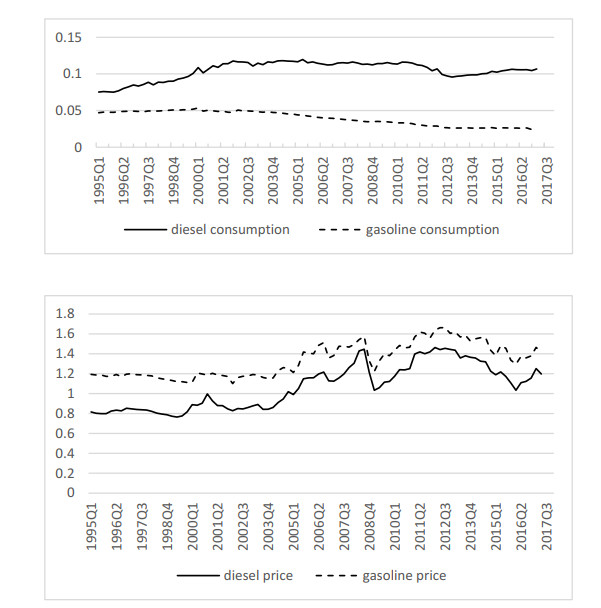
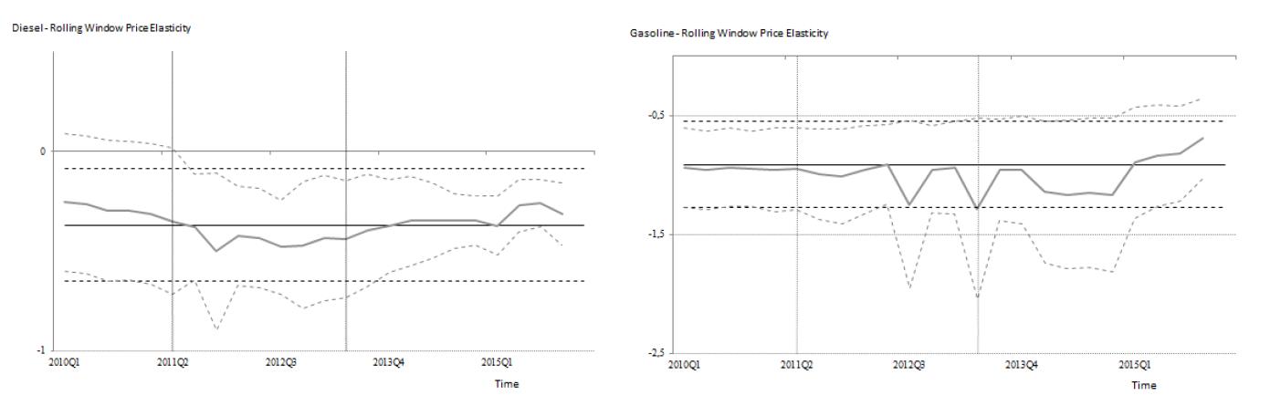
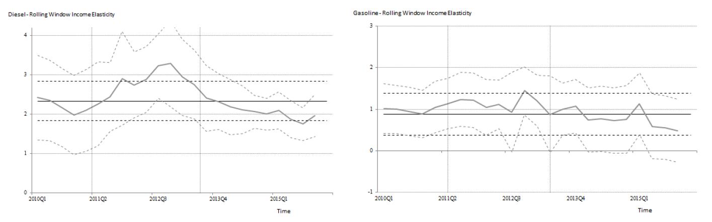
Despite the increase in electric mobility, fossil fuels still dominate the transport sector. For a sustainable management of these fuels, environmental policy plays a significant role. It is key to know if higher taxes are effective to moderate demand, which will depend on demand elasticities. While price elasticities determine the effectiveness of higher taxes, income elasticities are important for macroeconomic policy considerations. Furthermore, in dynamic societies and economies, it is possible that elasticities change over time or as a response to certain events, determining the need to adjust policies. We study the case of a small, open economy, highly dependent on fuel imports: Portugal. Our estimation of price and income elasticities for gasoline and diesel demand control for breakpoints and uses a dynamic perspective. The period covered (1995–2015) includes important macroeconomic events, such as the fuel market liberalization and a severe economic crisis. Results for the whole period show that long-run price elasticities are −0.368 for diesel and −0.911 for gasoline. Hence, taxes are more effective to moderate gasoline demand than diesel demand. Long-run income elasticities are 2.338 for diesel and 0.877 for gasoline, demonstrating the strong dependence of diesel consumption on the level of economic activity. The breakpoint analysis indicates that contrarily to the fuel market liberalization process, the economic crisis impacted elasticities. Furthermore, we find variability in elasticities around the period of the economic crisis, which justifies the need for a flexible policy. Dynamic policies can use specific periods as opportunities to promote technical and behavioral desirable changes.
Citation: Susana Silva, Isabel Soares, Carlos Pinho. Dynamic behavior of transport fuel demand and regional environmental policy: The case of Portugal[J]. AIMS Energy, 2021, 9(5): 899-914. doi: 10.3934/energy.2021042
Despite the increase in electric mobility, fossil fuels still dominate the transport sector. For a sustainable management of these fuels, environmental policy plays a significant role. It is key to know if higher taxes are effective to moderate demand, which will depend on demand elasticities. While price elasticities determine the effectiveness of higher taxes, income elasticities are important for macroeconomic policy considerations. Furthermore, in dynamic societies and economies, it is possible that elasticities change over time or as a response to certain events, determining the need to adjust policies. We study the case of a small, open economy, highly dependent on fuel imports: Portugal. Our estimation of price and income elasticities for gasoline and diesel demand control for breakpoints and uses a dynamic perspective. The period covered (1995–2015) includes important macroeconomic events, such as the fuel market liberalization and a severe economic crisis. Results for the whole period show that long-run price elasticities are −0.368 for diesel and −0.911 for gasoline. Hence, taxes are more effective to moderate gasoline demand than diesel demand. Long-run income elasticities are 2.338 for diesel and 0.877 for gasoline, demonstrating the strong dependence of diesel consumption on the level of economic activity. The breakpoint analysis indicates that contrarily to the fuel market liberalization process, the economic crisis impacted elasticities. Furthermore, we find variability in elasticities around the period of the economic crisis, which justifies the need for a flexible policy. Dynamic policies can use specific periods as opportunities to promote technical and behavioral desirable changes.

| [1] | BP (2017). BP energy outlook. |
| [2] |
Labandeira X, Labeaga J, López-Otero X (2017) A meta-analysis on the price elasticity of energy demand. Energy Policy 102: 549–568. doi: 10.1016/j.enpol.2017.01.002

|
| [3] | Sterner T (2006) Survey of transport fuel demand elasticities. Stockholm: The Swedish Environmental Protection Agency, Report 5586. |
| [4] | Graham J, Glaister S (2002) The demand for automobile fuel: A survey of elasticities. J Transp Econ Policy 36: 1–25. |
| [5] | Hanly M, Dargay J, Goodwin P (2002) Review of income and price elasticities in the demand for road traffic-Final Report. ESRC TSU publication 2002/13. |
| [6] |
Odeck J, Johansen K (2016) Elasticities of fuel and traffic demand and the direct rebound effects: An econometric estimation in the case of Norway. Transp Res Part A 83: 1–13. doi: 10.1016/j.trb.2015.11.013
|
| [7] | Boshoff W (2012) Gasoline, diesel fuel and jet fuel demand in South Africa. J Stud Econ Econ 36: 43–78. |
| [8] | Frondel M, Vance C (2014) More pain at the diesel pump? An econometric comparison of diesel and petrol price elasticities. J Transp Econ Policy 48: 449–463. |
| [9] |
Pock M (2010) Gasoline demand in Europe: New insights. Energy Econ 32: 54–62. doi: 10.1016/j.eneco.2009.04.002
|
| [10] |
Akinboade O, Ziramba E, Kumo W (2008) The demand for gasoline in South Africa: An empirical analysis using co-integration techniques. Energy Econ 30: 3222–3229. doi: 10.1016/j.eneco.2008.05.002
|
| [11] | Park S, Zhao G (2010) An estimation of U.S. gasoline demand: a smooth time-varying cointegation approach. Energy Econ 32: 110–120. |
| [12] |
Baranzini A, Weber S (2013) Elasticities of gasoline demand in Switzerland. Energy Policy 63: 674–680. doi: 10.1016/j.enpol.2013.08.084
|
| [13] |
Alves D, Bueno R (2003) Short-run, long-run and cross elasticities of gasoline demand in Brazil. Energy Econ 25: 191–199. doi: 10.1016/S0140-9883(02)00108-1
|
| [14] |
Cheung KY, Thomson E (2004) The demand for gasoline in China: a cointegration analysis. J Appl Stat 31: 533–544. doi: 10.1080/02664760410001681837
|
| [15] | Danesin A, Linares P (2015) An estimation of fuel demand elasticities for Spain: an aggregated panel approach accounting for diesel share. J Transp, Econ Policy 49: 1–16. |
| [16] | González-Marrero R, Lorenzo-Alegría R, Marrero G (2012) A dynamic model for road gasoline and diesel consumption: an application for Spanish regions. Int J Energy Econ Policy 2: 201–209. |
| [17] |
Bakhat M, Labandeira X, Labeaga J, et al. (2017) Elaticities of transport fuel at times of economic crisis: as empirical analysis for Spain. Energy Econ 68: 66–80. doi: 10.1016/j.eneco.2017.10.019
|
| [18] |
Bentzen J, Engsted T (1993) Short- and long-run elasticities in energy demand. Energy Econ 15: 9–16. doi: 10.1016/0140-9883(93)90037-R
|
| [19] |
Ben Sita B, Marrouch W, Abosedra S (2012) Short-run price and income elasticity of gasoline demand: Evidence from Lebanon. Energy Policy 46: 109–115. doi: 10.1016/j.enpol.2012.03.041
|
| [20] |
Hughes J, Knittel C, Sperling D (2008) Evidence of a shift in the short-run price elasticity of gasoline demand. Energy J 29: 113–134. doi: 10.5547/ISSN0195-6574-EJ-Vol29-No1-9
|
| [21] |
Neto D (2012) Testing and estimating time-varying elasticities of Swiss gasoline demand. Energy Econ 34: 1755–1762. doi: 10.1016/j.eneco.2012.07.009
|
| [22] | Sterner T, Dahl C, Franzén M (1992) Gasoline tax policy, carbon emissions and the global environemnt. J Transp Econ Policy 26: 109–119. |
| [23] |
Sterner T (2007) Fuel taxes: An important instrument for climate policy. Energy Policy 35: 3194–3202. doi: 10.1016/j.enpol.2006.10.025
|
| [24] | Pesaran M, Shin Y (1998) An autoregressive distributed-lag modelling approach to cointegration analysis. In Econometrics and Economic Theory in the 20th Century. The Ragnar Frisch Centennial Symposium, ed. S. Strøm, chap. 11,371–413. Cambridge: Cambridge University Press. |
| [25] |
Pesaran M, Shin Y, Smith R (2001) Bounds testing approaches to the analysis of level relationships. J Appl Econ 16: 289–326. doi: 10.1002/jae.616
|
| [26] |
Polemis M (2006) Empirical assessment of the determinants of road energy demand in Greece. Energy Econ 28: 385–403. doi: 10.1016/j.eneco.2006.01.007
|
| [27] |
Eltony M, Al-Mutairi N (1995) Demand fos gasoline in Kuwait: An empirical analysis using cointegration techniques. Energy Econ 17: 249–253. doi: 10.1016/0140-9883(95)00006-G
|
| [28] |
Wu JH, Huang YL, Liu CC (2011) Effects of floating pricing policy: and application of system dynamics on oil market after liberalization. Energy Policy 39: 4235–4252. doi: 10.1016/j.enpol.2011.04.039
|
| [29] | Fattouh B, Oliveira C, Sem A (2015) Gasoline and diesel pricing reforms in the BRIC countries: a comparison of policy and outcomes. The Oxford Institute for Energy Studies, WPM 57. |
Figures(3) / Tables(7)

Susana Silva, Isabel Soares, Carlos Pinho. Dynamic behavior of transport fuel demand and regional environmental policy: The case of Portugal[J]. AIMS Energy, 2021, 9(5): 899-914. doi: 10.3934/energy.2021042


 DownLoad: