Research article

The probabilistic load flow analysis by considering uncertainty with correlated loads and photovoltaic generation using Copula theory

  • In this paper, a probabilistic load flow analysis is proposed in order to deal with probabilistic problems related to the power system. Due to increasing trend of penetration of renewable energy sources in power system brought two factors: One is uncertainty, and another one is dependence. Uncertainty and dependence factor increase risk associated with power system operation and planning. In this proposed model these two factors is considered. Gaussian Copula theory is proposed to establish the probability distribution of correlated input random variables. Three sampling methods are used with Monte Carlo simulation as simple random sampling, Box-Muller sampling, and Latin hypercube sampling in order to evaluate the accuracy of the proposed method. The main advantages of this model are as: It can establish any type of correlation between input random variable with the help of Copula theory, it is free from the restrictions of Pearson coefficient of correlation, it is unconstrained by the marginal distribution of input random variables, and uncertainty is established with photovoltaic generation this is the main source of uncertainty. Additional, in order to evaluate the accuracy and efficiency of the proposed model a real load and photovoltaic generation data is adopted. For accuracy evaluation purpose two comparative test system is adopted as modified IEEE 14 and IEEE 118-bus test system.

    Citation: Li Bin, Muhammad Shahzad, Qi Bing, Muhammad Ahsan, Muhammad U Shoukat, Hafiz MA Khan, Nabeel AM Fahal. The probabilistic load flow analysis by considering uncertainty with correlated loads and photovoltaic generation using Copula theory[J]. AIMS Energy, 2018, 6(3): 414-435. doi: 10.3934/energy.2018.3.414

    Related Papers:

    [1] Andrés Feijóo, Daniel Villanueva . Polynomial approximations of the Normal toWeibull Distribution transformation. AIMS Energy, 2014, 2(4): 342-358. doi: 10.3934/energy.2014.4.342
    [2] Muti Ur Rehman Tahir, Adil Amin, Ateeq Ahmed Baig, Sajjad Manzoor, Anwar ul Haq, Muhammad Awais Asgha, Wahab Ali Gulzar Khawaja . Design and optimization of grid Integrated hybrid on-site energy generation system for rural area in AJK-Pakistan using HOMER software. AIMS Energy, 2021, 9(6): 1113-1135. doi: 10.3934/energy.2021051
    [3] V. V. Thang, Thanhtung Ha . Optimal siting and sizing of renewable sources in distribution system planning based on life cycle cost and considering uncertainties. AIMS Energy, 2019, 7(2): 211-226. doi: 10.3934/energy.2019.2.211
    [4] Sulabh Sachan . Integration of electric vehicles with optimum sized storage for grid connected photo-voltaic system. AIMS Energy, 2017, 5(6): 997-1012. doi: 10.3934/energy.2017.6.997
    [5] K. M. S. Y. Konara, M. L. Kolhe, Arvind Sharma . Power dispatching techniques as a finite state machine for a standalone photovoltaic system with a hybrid energy storage. AIMS Energy, 2020, 8(2): 214-230. doi: 10.3934/energy.2020.2.214
    [6] Matteo Moncecchi, Davide Falabretti, Marco Merlo . Regional energy planning based on distribution grid hosting capacity. AIMS Energy, 2019, 7(3): 264-284. doi: 10.3934/energy.2019.3.264
    [7] Jin H. Jo, Zachary Rose, Jamie Cross, Evan Daebel, Andrew Verderber, John C. Kostelnick . Application of Airborne LiDAR Data and Geographic Information Systems (GIS) to Develop a Distributed Generation System for the Town of Normal, IL. AIMS Energy, 2015, 3(2): 173-183. doi: 10.3934/energy.2015.2.173
    [8] Alemayehu T. Eneyaw, Demiss A. Amibe . Annual performance of photovoltaic-thermal system under actual operating condition of Dire Dawa in Ethiopia. AIMS Energy, 2019, 7(5): 539-556. doi: 10.3934/energy.2019.5.539
    [9] Virendra Sharma, Lata Gidwani . Optimistic use of battery energy storage system to mitigate grid disturbances in the hybrid power system. AIMS Energy, 2019, 7(6): 688-709. doi: 10.3934/energy.2019.6.688
    [10] Awatif Nadia, Abdul Hasib Chowdhury, Esheta Mahfuj, Md. Sanwar Hossain, Khondoker Ziaul Islam, Md. Istianatur Rahman . Determination of transmission reliability margin using AC load flow. AIMS Energy, 2020, 8(4): 701-720. doi: 10.3934/energy.2020.4.701
  • In this paper, a probabilistic load flow analysis is proposed in order to deal with probabilistic problems related to the power system. Due to increasing trend of penetration of renewable energy sources in power system brought two factors: One is uncertainty, and another one is dependence. Uncertainty and dependence factor increase risk associated with power system operation and planning. In this proposed model these two factors is considered. Gaussian Copula theory is proposed to establish the probability distribution of correlated input random variables. Three sampling methods are used with Monte Carlo simulation as simple random sampling, Box-Muller sampling, and Latin hypercube sampling in order to evaluate the accuracy of the proposed method. The main advantages of this model are as: It can establish any type of correlation between input random variable with the help of Copula theory, it is free from the restrictions of Pearson coefficient of correlation, it is unconstrained by the marginal distribution of input random variables, and uncertainty is established with photovoltaic generation this is the main source of uncertainty. Additional, in order to evaluate the accuracy and efficiency of the proposed model a real load and photovoltaic generation data is adopted. For accuracy evaluation purpose two comparative test system is adopted as modified IEEE 14 and IEEE 118-bus test system.


    1. Introduction

    Currently, the electric power system is confronting many uncertainties. The main source of these uncertainties is penetration of renewable energy sources in power system network. Among these renewable energy sources, photovoltaic (PV) generation and wind energy generation are the dominant sources of uncertainty. Due to randomness nature of uncertainty, it increases the risk associated with electric power system operation modes and further has an influence on load flow analysis. Most of these uncertainties are dependent. This dependence relationship can be linear or non-linear. For example, the loads in the same area can be increased or decrease in a same time due to environmental and social ones. Similarly, the output power of wind energy sources is strongly correlated with the wind speed of neighboring measuring stations [1,2]. On the other hand, the power system highly uncertain due to changing pattern of power demand like the transport (electric mobility) and heat sectors (heat pumps in buildings) [1]. Safeguarding the reliability of the power system is a key enabler for this massive system transformation. For the operation of future power systems, new methods are needed to incorporate the different sources of uncertainty (contingencies, load and renewable energy source forecast errors) during the operational planning stage and to help system operators to steer the system into risk-averse modes of operation [3,4,5].

    The probabilistic load flow (PLF) analysis is a tool that can handle uncertainties in the efficient and effective way. The PLF is a steady-state load flow analysis to determine the network parameters by considering uncertainty with input random variables flexibly. The information obtained by PLF analysis is used for power system security assessment, operation and control purpose. In literature, many PLF methods have been used in order to deal with correlated input random variables. In these methods included: Gaussian mixture model method [6,7,8], point estimation method [9,10,11], convolution method [12,13], cumulant method [8,14], unscented transformation [15], and Monte Carlo simulation (MCS) [16,17,18,19]. MCS methods are the most popular methods among all of above methods. It is due to its simplicity and ability to handle complex non-linear problems. Most of the above methods only deal with a linear dependence. Additional, the Persons linear correlation coefficient has been used for measuring the degree of dependence. Most of the nature uncertainties are not linear. This proposed model can handle this non-linear dependence more flexible.

    All methods used for PLF can be divided into four categories. These categories are as numerical methods, analytical methods, approximate methods, and hybrid methods [20]. A numerical MCS method with simple random sampling (SRS) has been used frequently for PLF power system problems. MCS with SRS can be express as SMCS. SMCS method has been used as a reference for accuracy comparison in PLF studies [5,8,10,15,21,22,23,24]. From the literature, it is clear that no one method is more accurate than SMCS in term of accuracy. However, it suffers heavy computational burden to achieve the desired accuracy. To overcome computational burden, in literature many methods have been used such as convolution techniques [12,13]. The convolution base methods are also time-consuming due to discrete point problems. Point estimation based methods have lesser computational burden but less accurate. In fact, there are no holistic criteria for PLF evaluation. Always there is a compromise between computational burden and accuracy. But currently, a third moment has been started to overcome computational burden and accuracy problems. This moment is to hybrid methods like combined cumulants and Laplace transform method [25], combine cumulant and Gaussian mixture method [8], cumulant and multiple integral method [26], second order design method [17]. Actually, the accuracy and computational burden of PLF methods highly depend upon the modelling of input uncertainty and sampling techniques.

    The contribution in this research work has many aspects included: Almost all of the methods in literature can only deal with a linear correlation between input random variables and have been considered Pearson linear correlation coefficient. This Pearson linear correlation coefficient some time cannot measure the degree of correlation. For example: 1) it cannot measure non-linear dependence between input random variable; 2) it can't measure dependence for those distributions that have not define standard deviation; 3) it is invariant under strictly increasing transformation. To overcome this problem in this work Gaussian Copula theory is proposed that can handle linear and non-linear problems flexibly. By using Copula theory, a desirable correlation can be achieve between input random variables. The other aspect of this work is modelling of input uncertainty. The PV generation and correlated load are used for modelling the input uncertainty. The special in this work real data about PV generation and load are used for accuracy comparison purpose. Additional, the Box-Muller sampling (BMS) and Latin hypercube sampling (LHS) are used for accuracy and computational burden comparison purpose. The SMCS is used for a benchmark for other methods in term of accuracy and computational burden. MCS combine with BMS can be express as BMCS and MCS combine with LHS can be express as LMCS. For three methods, Copula theory is used for capturing the complex stochasticity of correlated loads and PV generation. The modified IEEE 14-bus and IEEE 118-bus test system is used for obtaining results.

    The paper is organized as follows. Section 2 describes the modelling of the probability distribution of input random variable included correlated loads and correlated PV generation. Section 3 describes the methodology, and sampling techniques included SRS, BMS, and LHS. Section 4 describes the PLF analysis procedure. Section 5, evaluate the performance analysis of proposed methods. Finally, conclusions are drawn in Section 6.


    2. Modelling of input random variables for uncertainty

    The accuracy and computational efficiency of PLF analysis usually depending upon three major factors included: a) Uncertainty handing method; b) Accurate power system model; c) Accurate modelling input random variable uncertainty.


    2.1. Modelling of correlated loads for uncertainty

    There are normally two methods for measurement of correlation between random variable with respect to degree and structure. First one is Pearson's linear correlation coefficient that can only measure the degree of correlation Eq 1. The second one is rank correlation coefficient and Copula theory that can measure the degree as well as the structure of correlation. In this work, Copula theory is proposed to measure the structure as well as the degree of correlation between random variables flexibly. This theory can measure the linear and non-linear correlation between random variables. More, it is invariant under strictly increasing transformation. The correlation matrix for n input random variable is shown in Eq 1 as:

    Cor_matrix=[1ρ21...ρ1nρ211...ρ2nρn1ρn2...1] (1)

    Where ρij is the correlation coefficient and can be calculated as ρij=cov(Wi,Wj)/σiσj where σi and σj is the standard deviation of a random variable Wi and Wj respectively and cov(Wi,Wj) is the covariance. According to Copula theory, it can be express as in Eq 2 for bivariate:

    F12(w1,w2)=C(F1(w1),F2(w2)) (2)

    Where C is a copula function, according to Sklar theorem [27]. It couples multivariate joint distribution CDF to one dimensional marginal CDFs. F1(w1) and F2(w2) are the marginal CDF of two random variables W1 and W2 respectively. F12(w1,w2) is the joint CDF of these two random variables. C(F1(w1),F2(w2)) is the Copula density function, and it must follow the Sklar theorem property as mention in Eq 3:

    U[0,1]:P(Uu)=P(F(w)u)=P(wF1(u))=F[F1(u)]=u (3)

    It can be extended to multivariate as in Eq 4, m is the number of random variables:

    f(w1,...,wm)=c(F1(w1),...,Fm(wm)).mi=1fi(wi) (4)

    Where C(F1(w1),..,Fm(wm))=mC(F1(w1),..,Fm(wm))F1(w1).........Fm(wm) is the Copula density function for multivariate random variables.

    There are many Copula families, but famous one is included elliptical Copula and Archimedean Copula. Here, Gaussian Copula is proposed to measure the dependence between input random variables that belong to Archimedean Copula family. All loads PDFs are modelled as a Gaussian distribution follows the Eq 5:

    f(x;μ;σ)=12πσe((xμ)22σ2) (5)

    Where x is the required value for which probability distribution function (PDF) needed, μ is the mean value of the load, and σ is the arbitrary value of standard deviation. To show the accuracy of modelled load PDF is compare with actual one day load at MAISY utility customer energy use with per hourly interval available in [28]. Figure 1 shows the PDFs and CDFs of real, generated, and ideal data of loads. Gaussian Copula function is used to establish the desired correlation between different random variables (loads) in the proposed network. The PDFs of multivariate Gaussian distribution with desirable correlation can be found by Eq 6.

    Figure 1. Probability density function (PDF) and Cumulative density function (CDF) of real, generated, and ideal data for loads are shown in (a) and (b) respectively.
    CGaussR(u)=1det.Rexp(12(ϕ1(u1)....................ϕ1(ud))T.(R1I).(ϕ1(u1)....................ϕ1(ud))) (6)

    Where R is the correlation matrix belong to [1,1]d×d, C show the correlation density function, ϕ1 is the inverse CDF of standard normal distribution, u1,.........,ud is the random variables, d is the number of variables, and I is the identity matrix. The correlation of bivariate function over unit domain from weak to strongly correlated loads with the help of Gaussian Copula is shown in Figure 2.

    Figure 2. Scatter plots of correlated loads in unit domain (a) ρ = 0.6; (b) ρ = 0.8; (c) ρ = 0.9; (d) ρ = 0.99.

    2.2. PV generation modelling for uncertainty

    In this work, PV generations are model as a beta distribution with the help of Eq 7. The historical solar power data for integration studies located at California western state is taken to check the accuracy of modelled PV generation available at National Renewable Energy Laboratory (NREL) [29]. One day data (Jun 1, 2006) with a 5-minute interval is taken to check the accuracy of the proposed model.

    f(x;,α,β)=Γ(α+β)Γ(α)Γ(β)xα1(1x)β1 (7)

    Where x is the observed values or realization, α and β are the shape parameters and always α, β > 0, Ґ is the gamma function. The PDFs and CDFs of real, generated, and ideal values model with the help of Eq 7 are shown in Figure 3.

    Figure 3. Probability density function (PDF) and Commutative density function (CDF) of PV generation with real, generated, and ideal data are shown in (a) and (b) respectively.

    3. Methodology

    Monte Carlo Simulation is an iterative approach, mostly used for probabilistic load flow analysis. In this approach cumulative distribution function is prepared of a random variable to obtain the uncertainty. To model, the CDF of a random variable is an essential step in this approach. Accurate modelling of CDF give the accurate final results. In this numerical approach, in order to model the uncertainty as a random variable, three basic steps are needed as shown in Figure 4: (1) to model CDF of random variable; (2) to solve the deterministic load flow model; (3) statistical analysis of results.

    Figure 4. Monte Carlo Simulation steps.

    Monte Carlo Simulation process can be described by Eq 8:

    Y=h(X) (8)
    X=[X1,.....,Xn]T (9)
    Y=[Y1,......,Yn]T (10)

    Where in Eq 8–10, X is the vector of input random variable, Y is a vector of output random variables vector, and h is the function of the model under study. The object of study is to obtain PDF of Y at given known PDF of X. T shows the transpose.


    3.1. Simple random sampling

    Simple random sampling techniques is a theoretical basis technique to design other methods. The variance of the mean of output variable is calculated to find the robustness of sampling techniques [30]. The mean of the sample is calculated as in Eq 11:

    _y=1NNi=1yi (11)

    Where N is the number of samples, ˉy is the expected value and yi is the output value of ith iteration. The variance of the sample can be obtained as in Eq 12:

    var(y)=1NNi=1(yi_y)2 (12)

    The variance of the estimating mean can be determined by Eq 13:

    var(_y)=1Nvar(y) (13)

    3.2. Box-Muller sampling

    Box-Muller sampling is also as a sampling technique. In order to determine the sample of given iteration, firstly two random number from uniform distribution in the range of (0, 1) is generated. The sample should be determined by following Eq 14:

    Si=μi+cos(2πu1)×σi2ln(u2) (14)

    Where, Si = is the ith sample; µ = mean value of random variable; σ = standard deviation of a random variable; u1 & u2 = uniformly distributed random number in range of (0, 1). For the proposed PLF model, µi and σi are the base load and standard deviation for input variable.


    3.3. Latin hypercube sampling

    Latin hypercube sampling (LHS) is the type of stratified sampling. It uses to generate a sample of a random variable from entire distribution. In this technique, random variable distribution is divided into equal probability distribution intervals. Each interval is sample exactly once in its entire range of the random variable. In this way, sample value represents the higher sampling efficiency. The sampling procedure is as follows:

    Yn=Fn(Gn) (15)

    Where in Eq 15, Yn is the CDF of N input random variables such that Gn=G1,........,GN in probability theory, in range Yn = [0, 1]. If the sample size is denoted by K. If the entire range of YN is divided into k non-overlapping intervals than each interval length is equal to 1/k as shown in Figure 5. The sample value is generated from each interval without replacement randomly or midpoint value. In this work, midpoint value is chosen, and this method is call lattice sampling. The sampling value of Gn can be computed by taking the inverse function of Eq 16. The nth sample can be computed as in Eq 16:

    Figure 5. Illustration of latin hypercube sampling procedure.
    Gnk=F1n(n0.5k) (16)

    The sample values of Gn can be assembled as in Eq 17 in the row of sampling matrix:

    [Gn1,.......,GnN] (17)

    From this procedure, the n × k matrix can be obtained.

    As described in Section 3.1 the robustness of sampling techniques can be measure on the mean output statistic [30]. Therefore, the mean and variance can be computed by using Eq 11 and Eq 12 respectively. The variance of the estimated mean can be computed with the help of Eq 18:

    Var(_y)=1Nvar(y)N1Ncon(G1,G2) (18)

    Where con(G1,G2) is the covariance between random variables.


    4. Probabilistic load flow evaluations

    The deterministic load flow analysis can be described by Eq 19:

    Y=h(X) (19)

    Where X is the input vector of nodal active and reactive power injections. Y is the output vector of voltage (V), voltage phase angle (θ), active load flow (Pij), reactive load flow (Qij), h(X) is the load flow function [31]. In case of PLF analysis, correlated nodal loads, PV generation, and conventional generator are the input random variable with their probability distribution functions. The statistical distribution of output variables V, θ, P, and Q are calculated. There are following steps used to perform PLF analysis:

    ●  Prepare the CDF of model correlated loads and correlated PV generations, to set all basic requirement for deterministic load flow analysis, e.g. sample size N.

    ●  To determine the input random variables G.

    ●  To select the desire sampling procedure.

    ●  To generate the sample matrix N × k.

    ●  To set the initial starting point n = 1.

    ●  To perform the deterministic load flow analysis and obtain the values of V, θ, P, Q.

    ●  Set n=n+1; if n<N go to step 6. Otherwise, go to next step.

    ●  To do a statistical analysis of output random variable V, θ, P, Q.


    5. Performance evaluation of proposed methods

    A series of PLF analysis is carried out to determine the performance of SMCS, BMCS, and LMCS. The PLF analysis is carried out on modified IEEE 14-bus test system and IEEE 118-bus test system. The program is developed with "DIgSILENT PowerFactory (15.1) platform. The simulation was performed on PC with AMD A12-9700P, RADEON R7, 10 COPMPUTE CORES UC+6G, 2.5 GHZ processing speed, and 8 GB RAM". The results obtained by the proposed method are compared with correlated SMCS.

    To determine the accuracy of proposed model two error indices are introduced in Eq 20 and Eq 21 [9,10] are adopted.

    εμ=|μaccμproμacc|×100% (20)
    εσ=|σaccσproσacc|×100% (21)

    Where εμ is an error of the output random variables with * category (* represents V, θ, P, and Q). Second εσ is an error of standard deviation with the * category. The results obtained by the SRS method with a sample size of 20,000 are assumed to be accurate and benchmark. The mean and standard deviation of SMCS method are express as µacc and σacc respectively. Similarly, the mean and standard deviation of proposed methods are express as µpro and σpro respectively. ˉεμ and ˉεσ are the average error index and average standard deviation error index that determined the distribution convergence of entire system.

    To evaluate the convergence of two methods, each method is run 100 times with certain sample size. In this way, 100 values of εμ and εσ are calculated with four variable categories. For 100 times calculation, two indices are introduced. First one is the mean of the standard deviation error. The second one is the mean of a maximum of error. The standard deviation error is the standard deviation error obtain from 100 calculations for each output categories and denoted by εσ100. The mean of the standard deviation error is the mean of εσ100 each specific type of output random variables and denoted by ˉεσ100. This ˉεσ100 show the stability of two methods. The maximum error of each output random variables are calculated in term of its mean and standard deviation. The mean of maximum of error is calculated is express as ˉεμ,max for each output categories. Similarly, mean of the maximum of error standard deviation is calculated and denoted by ˉεσ,max for each output random variable is calculated. For example, let V1,......,Vn is the voltage magnitude of the n node test system and ε1μVi,......,ε100μVi be the error of Vi after 100 calculationsi=1,.....,n. ThenεViμ,max=max{ε1μVi,.......,ε100μVi},i=1,......,n. For voltage variable mean of the maximum of error is calculated as εVμmax=1nni=1εViμmax. Similarly, other variable statistic can be obtain.


    5.1. The modified IEEE 14-bus test system

    All deterministic load flow data about this test system is available in [32]. The modified IEEE 14-bus test system is shown in Figure 6. There are total 23 input random variables in this test system. The load distribution is followed Gaussian distribution and discrete, and generator output follows the binomial distribution. The PLF analysis with 20,000 times MCS with SRS sampling consider to be the benchmark for other two methods and consider to be accurate and use to determine the error for other methods as it is usual practice in PLF study [9,10]. Two kinds of correlation is adopted in this test system. First one is between load and other is between active power outputs of PV generations. The constant power factor load model is adopted. The detail load parameters are presented in Table 1.

    Figure 6. Modified IEEE 14-bus test system.
    Table 1. Parameters of loads.
    Node No. Mean (p.u) StdDev (p.u) Power Factor
    2 0.215 0.065 0.864
    3 0.943 0.031 0.991
    4 0.481 0.115 0.365
    5 0.074 0.036 0.978
    6 0.111 0.037 0.833
    9 0.295 0.156 0.872
    10 0.094 0.036 0.823
    11 0.036 0.015 0.889
    12 0.061 0.024 0.965
    13 0.134 0.048 0.919
    14 0.151 0.062 0.949
     | Show Table
    DownLoad: CSV

    All loads are divided into three groups as G1={2,3,4,5,6}, G2={10,11,12,13,14} and {9}. The correlation matrix between G1 is presented in Eq 22 and correlation matrix between G2 is presented in Eq 23. The correlation between same group loads is dependent as shown in Eq 22 and Eq 23 and also correlation between different load groups also dependent with 0.5 correlation coefficient.

    G1=[10.60.70.50.70.610.70.60.80.70.710.70.80.50.60.710.70.70.80.80.71] (22)
    G2=[10.60.70.50.70.610.70.60.80.70.710.70.80.50.60.710.70.70.80.80.71] (23)

    Load 9 is correlated with active power output of PV generation available at node 9 with correlation coefficient 0.6. Two PV generation is located at node 9 with installed capacity 0.1 p.u, the active power of PV generation follow the Eq 7 and reactive power assumed to be zero [33,34]. The correlation coefficient matrix between two PV generation and load 9 is presented in Eq 24.

    GPVL9=[10.90.60.910.60.60.61] (24)

    The simulation is change from 100 to 1000 with step size 100. In order to evaluate the performance of SMCS, BMCS, and LMCS error curve are adopted. All the error indices are calculated for all type of output random variables included voltage magnitude, phase angle, active power, and reactive power. The error indices of only active power are consider for presenting the results for all four categories of variables.


    5.2. Simulation results analysis of IEEE 14-bus test system

    In the simulation analysis, three types are error indices are calculated as average error, mean of the maximum error, and mean of the standard deviation error indices. The average error index determines the distribution convergence degree of the entire system with corresponding output random variable. The other two error indices as mean of the standard deviation error and mean of the maximum of error are determine the stability of the entire method. For obtaining these error indices simulation is performed 100 times for 1000 samples with 100 step size.

    The results of Figure 7 (ac) illustrate the mean of the maximum of error curves with three methods. To present the results only active power through the line 2–3 was considered for IEEE 14-bus test system. It shows the percentage of the mean of maximum of error for 100 sample size to 1000 sample size with 100 step size of three methods SMCS, BMCS, and LMCS. The mean of the maximum of error of three methods SMCS, BMCS, and LMCS was almost 4.88%, 3.56%, and 0.96% respectively with 100 sample size. Similarly, this error index was 2.15%, 1.16%, 0.15% with 1000 sample size. This error index promptly reduces at 200 sample size, after 200 sample size it remains almost constant. Finally, the results of Figure 7 (ac) shows that LMCS method is more stable method than other two methods. The results of Figure 7 (df) illustrate the average error index for three methods. Form these results, it is clearly shown that the LMCS has 0.10% error, but the other two method SMCS and BMCS have 0.71% and 0.58% respectively with 1000 sample size. This show that the LMCS method is best convergence degree for proposed test system rather than other two methods. The results of Figure 7 (gi) illustrate the mean of the standard deviation error. This show that the LMCS has 0.11% error and other two methods have 0.42% and 0.32% respectively with 1000 sample size. Form these results, it is clearly shown that the LMCS is more stable method than the other two methods.

    Figure 7. Mean of the maximum error (a–c), average error indices (d–f), and mean of the standard deviation error (g–i) curves for active power through the line 2–3 for corresponding method.

    The standard deviation error indices are presented in Figures 8 (ai). The mean of maximum error of standard deviation is presented in Figure 8 (ac), average of standard deviation error index is in Figure 8 (df), and mean of standard deviation error is in Figure 8 (gi). All of these indices are calculated with 1000 sample size. The mean of maximum of standard deviation error index of LMCS method was with 1.49%, but the SMCS and BMCS have 3.36% and 2.23%. Similarly, average standard deviation error index of LMCS was 0.40%, but the SMCS and BMCS have 2.23% and 0.44%. Similarly, mean of standard deviation error index of LMCS was 0.16%, but the SMCS and BMCS have 0.28% and 0.20%. All of these results prove that LMCS method is much better than SMCS but almost identical to BMCS method according to distribution convergence and stable point of view.

    Figure 8. Mean of maximum standard deviation error (a–c), average standard deviation error indices (d–f), and mean of standard deviation error (g–i) curves for active power through the line 2–3 for corresponding method.

    All of the above calculated error indices are for active power output random variable. The remaining three output random variables, i.e. voltage magnitude, phase angle, and reactive power error indices are very similar to this. These are not shown here due to space limitations. All of the remaining output random variable's error indices are calculated and presented in Table 2 with sample size 400. The results of Table 2 show that error indices of all output variable are within 10% with SMCS but with BMCS and ILMCS are within 5%. Additional, the PDF and CDF of active power flow through the line 2–3 are illustrated in Figure 9. From the results of Figure 9, shows that the curves are very close to each other for three methods. All of these curves are calculated with a different sample sizes like SMCS with 20,000 samples and BMCS, and LMCS are with 1000 samples. The accuracy of presented results is almost same but BMCS and LMCS with 1000 sample size. The computational time comparison of three methods is shown in Figure 10. The computational time of SMCS method with sample size 20,000 was 981 s seconds. The computational time for both BMCS and LMCS was almost same like 3.17 s but with 1000 sample size. The computational burden of LMCS was very small for desire accuracy. The results of Figure 10 shows the computational superiority of ILHS with respect to same sample size.

    Table 2. Error comparison of IEEE 14-bus test system.
    Method SMCS BMCS LMCS Method SMCS BMCS LMCS
    εvμ(%) ˉεvμ,max 1.022 0.018 0.012 εPijμ(%) ˉεpμ,max 2.151 1.164 0.156
    ˉεvμ 1.042 0.037 0.016 ˉεpμ 0.717 0.852 0.104
    ˉεvσ100 0.451 0.021 0.019 ˉεpσ100 0.421 0.323 0.115
    εvσ(%) ˉεvσ,max 6.451 1.882 1.667 εPijσ(%) ˉεpσ,max 3.365 2.235 1.490
    ˉεvσ 2.957 0.924 0.863 ˉεpσ 2.235 0.447 0.406
    ˉεvσ100 1.675 0.643 0.573 ˉεpσ100 0.285 0.201 0.167
    εθμ(%) ˉεθμ,max 3.056 1.568 1.235 εQijμ(%) ˉεQμ,max 5.689 2.235 2.035
    ˉεθμ 1.023 0.756 0.583 ˉεQμ 2.865 1.356 1.128
    ˉεθσ100 0.982 0.458 0.394 ˉεQσ100 1.225 0.754 0.586
    εθσ(%) ˉεθσ,max 9.985 3.895 3.128 εQijσ(%) ˉεQσ,max 9.972 3.365 2.864
    ˉεθσ 3.458 1.358 1.023 ˉεQσ 4.258 2.235 2.078
    ˉεθσ100 2.896 0.886 0.748 ˉεQσ100 2.458 1.423 1.358
     | Show Table
    DownLoad: CSV
    Figure 9. robability density function (PDF) and cumulative density function (CDF) of active power flow through the line 2–3, (a) and (b) respectively, for three methods as: (a) SMCS, (b) BMCS, and (c) LMCS, for IEEE 14-bus test system.
    Figure 10. Computational time (seconds) comparison curve for three methods as: (a) SMCS, (b) BMCS, and (c) LMCS, for IEEE 14-bus test system.

    5.3. Modified IEEE 118-bus test system

    All of the deterministic data about this test system is available in [32] and also shown in Figure 13. All of the assumption and probabilistic data about this test system is same as in [10,31]. The total input random variables in this test system are 170. The reaming assumption are almost same as in previous test system like loads are follow normally distribution and generator output follow binomial distribution. Four PV generator are located at nodes 5, 16, 50, and 53, respectively with 0.2 p.u installed capacity. The correlation matrix of four PV generation is shown in Eq 25.

    GPVG4=[10.7000.71000010.7000.71] (25)

    5.4. The simulation results analysis of IEEE 118-bus test system

    By the simulation study, it is shown that the three types of error indices about four output variables categories were almost same pattern as in IEEE 14-bus test system. These indices are not presented here due to space limitations. The error indices of four categories are presented in Table 3 but with 800 sample size. The results of Table 3 show that the error indices of SMCS are within 10%, with BMCS are within 6%, with LMCS are within 4%. These percentage of error change due to increase input random variables. This conclusion shows that LMCS is more stable and distributed convergent method than the other two methods. The PDF and CDF curves are shown in Figure 11 of active power flow through the line 78–79. From these results, it is shown that LMCS is accurate than BMCS and SMCS but in previous test system BMCS was close to LMCS and SMCS methods. The accuracy of BMCS in term of PDF and CDF are bring down may be due to increase number of input random variables. Additionally, the comparison of the computational time of different sample same is shown in Figure 12. The computational time of SMCS method with sample size 20,000 was 5586 seconds. The computational time for both BMCS and LMCS was almost same like 13.92 s with 1000 sample size. The computational burden of BMCS and LMCS was very small as compare to SMCS for achieving desire accuracy. The results of Figure 12 show the computational superiority of ILHS with respect to same sample size.

    Table 3. Error comparison of IEEE 118-bus test system.
    Method SMCS BMCS LMCS Method SMCS BMCS LMCS
    εvμ(%) ˉεvμ,max 0.929 0.016 0.012 εPijμ(%) ˉεpμ,max 1.955 1.012 0.154
    ˉεvμ 0.947 0.032 0.016 ˉεpμ 0.652 0.741 0.103
    ˉεvσ100 0.410 0.018 0.019 ˉεpσ100 0.383 0.281 0.114
    εvσ(%) ˉεvσ,max 5.865 1.637 1.650 εPijσ(%) ˉεpσ,max 3.059 1.943 1.475
    ˉεvσ 2.688 0.803 0.854 ˉεpσ 2.032 0.389 0.402
    ˉεvσ100 1.523 0.559 0.567 ˉεpσ100 0.259 0.175 0.165
    εθμ(%) ˉεθμ,max 2.778 1.363 1.223 εQijμ(%) ˉεQμ,max 5.172 1.943 2.015
    ˉεθμ 0.930 0.657 0.577 ˉεQμ 2.605 1.179 1.117
    ˉεθσ100 0.893 0.398 0.390 ˉεQσ100 1.114 0.656 0.580
    εθσ(%) ˉεθσ,max 9.077 5.387 3.097 εQijσ(%) ˉεQσ,max 9.065 5.926 2.836
    ˉεθσ 3.144 2.181 1.013 ˉεQσ 3.871 2.943 2.057
    ˉεθσ100 2.633 0.770 0.741 ˉεQσ100 2.235 1.237 1.345
     | Show Table
    DownLoad: CSV
    Figure 11. Probability density function (PDF) and cumulative density function (CDF) of active power flow through the line 78–79, (a) and (b) respectively, for three methods as: (a) SMCS, (b) BMCS, and (c) LMCS, for IEEE 118-bus test system.
    Figure 12. Computational time (seconds) comparison curves for three methods as: (a) SMCS, (b) BMCS, and (c) LMCS, for IEEE 118-bus test system.
    Figure 13. Modified IEEE 118-bus test system.

    6. Conclusion

    Due to increasing trend of penetration of renewable energy sources into power system has introduced the uncertainties and dependence factors. The modelling of input random variable for the study of uncertainties and dependence effect on power system operation and planning is a challenge for future. In this paper, a probabilistic load flow analysis is presented for correlated loads and photovoltaic generation. Uncertainty is created with correlated loads and photovoltaic generation. Gaussian Copula theory is proposed to establish the correlation between input random variables. Form the results; it has proved that Copula theory can establish correlation between input random variables flexibly and overcome the restriction of Pearson's correlation coefficient. Additional, it is unconstrained by the marginal distribution type of input random variables. Two methods of sampling has been proposed for analysis purpose. The results obtained by LMCS method is more accurate and efficient. When the input random variables were small, the results obtain by BMCS and LMCS almost have same accuracy and robustness. But when the input random variable has increased BMCS become less accurate as compare to LMCS. As an overall result, LMCS is an efficient sampling method for convergence for entire distribution of input random variable, almost independent of input random variable, and flexible too. The LMCS method has a large potential in order to deal with probabilistic problems with renewable energy sources especially penetration of photovoltaic generation in power system network.


    Acknowledgements

    This work is supported by the "National Key Research and Development Program (2016YFB0901104), the National Natural Science Foundation of China (51307051), the Fundamental Research Funds for the Central Universities (2014ZP03, 2015ZD01) and the Science and technology projects from State Grid Corporation".


    Author contributions

    Li Bin and Qi Bing conceived the research idea and designed the simulation setup; Muhammad Shahzad did the remaining work.


    Conflicts of interest

    The authors declare no conflict of interest.


    [1] Bechrakis DA, Sparis PD (2004) Correlation of wind speed between neighboring measuring stations. IEEE T Energy Conver 19: 400–406. doi: 10.1109/TEC.2004.827040
    [2] Villanueva D, Feijóo A, Pazos JL (2010) Correlation between power generated by wind turbines from different locations. Available from: http://proceedings.ewea.org/ewec2010/allfiles2/20_EWEC2010presentation.pdf.
    [3] Jong MD, Papaefthymiou G, Palensky P (2017) A framework for incorporation of infeed uncertainty in power system risk-based security assessment. IEEE T Power Syst 33: 613–621.
    [4] Kirschen D, Jayaweera D (2007) Comparison of risk-based and deterministic security assessments. IET Gener Transm Dis 1: 527–533. doi: 10.1049/iet-gtd:20060368
    [5] Zhang P, Lee ST (2004) Probabilistic load flow computation using the method of combined cumulants and Gram-Charlier expansion. IEEE T Power Syst 19: 676–682.
    [6] Nijhuis M, Gibescu M, Cobben S (2017) Gaussian mixture based probabilistic load flow for LV-network planning. IEEE T Power Syst 32: 2878–2886. doi: 10.1109/TPWRS.2016.2628959
    [7] Valverde G, Saric A, Terzija V (2012) Probabilistic load flow with non-Gaussian correlated random variables using Gaussian mixture models. IET Gener Transm Dis 6: 701–709. doi: 10.1049/iet-gtd.2011.0545
    [8] Prusty BR, Jena D (2016) Combined cumulant and Gaussian mixture approximation for correlated probabilistic load flow studies: A new approach. Csee J Power Energ Syst 2: 71–78. doi: 10.17775/CSEEJPES.2016.00024
    [9] Caramia P, Carpinelli G, Varilone P (2010) Point estimate schemes for probabilistic three-phase load flow. Electr Pow Syst Res 80: 168–175. doi: 10.1016/j.epsr.2009.08.020
    [10] Morales JM, Perez-Ruiz J (2007) Point estimate schemes to solve the probabilistic power flow. IEEE T Power Syst 22: 1594–1601. doi: 10.1109/TPWRS.2007.907515
    [11] Kloubert ML, Rehtanz C (2017) Enhancement to the combination of point estimate method and Gram-Charlier Expansion method for probabilistic load flow computations. PowerTech, IEEE Manchester 2017: 1–6.
    [12] Wang Y, Zhang N, Chen Q, et al. (2016) Dependent discrete convolution based probabilistic load flow for the active distribution system. IEEE T Sustain Energ 8: 1000–1009.
    [13] Zhang N, Kang C, Singh C, et al. (2016) Copula based dependent discrete convolution for power system uncertainty analysis. IEEE T Power Syst 31: 5204–5205. doi: 10.1109/TPWRS.2016.2521328
    [14] Cai D, Chen J, Shi D, et al. (2012) Enhancements to the cumulant method for probabilistic load flow studies. Pow Energ Soc Gen Meeting 59: 1–8.
    [15] Aien M, Fotuhi-Firuzabad M, Aminifar F (2012) Probabilistic load flow in correlated uncertain environment using unscented transformation. IEEE T Power Syst 27: 2233–2241. doi: 10.1109/TPWRS.2012.2191804
    [16] Fang S, Cheng H, Xu G (2016) A modified Nataf transformation-based extended quasi-monte carlo simulation method for solving probabilistic load flow. Electr Mach Pow Syst 44: 1735–1744. doi: 10.1080/15325008.2016.1173130
    [17] Ren Z, Koh CS (2013) A second-order design sensitivity-assisted Monte Carlo simulation method for reliability evaluation of the electromagnetic devices. J Electr Eng Technol 8: 780–786. doi: 10.5370/JEET.2013.8.4.780
    [18] Tang L, Wen F, Salam MA, et al. (2015) Transmission system planning considering integration of renewable energy resources. Pow Energ Eng Conf 2015: 1–5.
    [19] Ayodele TR (2016) Analysis of monte carlo simulation sampling techniques on small signal stability of wind generator-connected power system. J Eng Sci Technol 11: 563–583.
    [20] Prusty BR, Jena D (2017) A critical review on probabilistic load flow studies in uncertainty constrained power systems with photovoltaic generation and a new approach. Renew Sust Energ Rev 69: 1286–1302. doi: 10.1016/j.rser.2016.12.044
    [21] Morales JM, Baringo L, Conejo AJ, et al. (2010) Probabilistic power flow with correlated wind sources. Let Gener Transm Dis 4: 641–651. doi: 10.1049/iet-gtd.2009.0639
    [22] Usaola J (2010) Probabilistic load flow with correlated wind power injections. Electr Pow Syst Res 80: 528–536. doi: 10.1016/j.epsr.2009.10.023
    [23] Gupta N (2016) Probabilistic load flow with detailed wind generator models considering correlated wind generation and correlated loads. Renew Energ 94: 96–105. doi: 10.1016/j.renene.2016.03.030
    [24] Prusty BR, Jena D (2017) A sensitivity matrix-based temperature-augmented probabilistic load flow study. IEEE T Ind Appl 53: 2506–2516. doi: 10.1109/TIA.2017.2660462
    [25] Kenari MT, Sepasian MS, Nazar MS, et al. (2017) The combined cumulants and Laplace transform method for probabilistic load flow analysis. Let Gener Transm Dis.
    [26] Wu W, Wang K, Li G, et al. (2016) Probabilistic load flow calculation using cumulants and multiple integrals. Let Gener Transm Dis 10: 1703–1709. doi: 10.1049/iet-gtd.2015.1129
    [27] Nelsen RB (2007) An introduction to copulas. Springer Science & Business Media.
    [28] Market Analysis and Information System (MAISY). Utility Customer Energy Use & Hourly Load Databases. Available from: http://www.maisy.com/.
    [29] National Renewable Energy Laboratory (NREL). Obtain Solar Power data: Western State California. Available from: https://www.nrel.gov/grid/solar-power-data.html.
    [30] Macdonald IA (2009) Comparison of sampling techniques on the performance of Monte-Carlo based sensitivity analysis. Eleventh International IBPSA Conference, 992–999.
    [31] Yu H, Chung CY, Wong KP, et al. (2009) Probabilistic load flow evaluation with hybrid latin hypercube sampling and cholesky decomposition. IEEE T Power Syst 24: 661–667. doi: 10.1109/TPWRS.2009.2016589
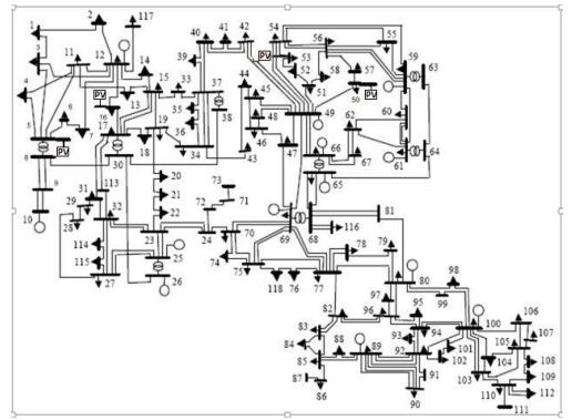
    [32] University of Washington Electrical Engineering: Power System Test Case Archive (January 2018). Available from: http://www.ee.washington.edu/research/pstca.
    [33] Karaki S, Chedid R, Ramadan R (1999) Probabilistic performance assessment of autonomous solar-wind energy conversion systems. IEEE T Energy Conver 14: 766–772. doi: 10.1109/60.790949
    [34] Reddy JB, Reddy DN (2004) Probabilistic performance assessment of a roof top wind, solar photo voltaic hybrid energy system. Rel Maint S-RAMS 2004: 654–658.
  • This article has been cited by:

    1. Angelo Raciti, Santi Agatino Rizzo, Giovanni Susinni, Circuit model of LED light bulb suitable for typical voltage THD on LV distribution networks, 2020, 212, 03787788, 109665, 10.1016/j.enbuild.2019.109665
    2. Muhammad Shahzad, Md. Rabiul Islam, Patrobers Simiyu, Nabeel Abdelhadi Mohamed Fahal, Muhammad Umair Shoukat, Khalid Hussain, 2018, Probabilistic Power Flow Model for the Uncertainty Analysis of Wind Energy and Loads, 978-1-5386-8524-2, 41, 10.1109/ICISET.2018.8745640
    3. Mahmoud G Hemeida, Salem Alkhalaf, Tomonobu Senjyu, Abdalla Ibrahim, Mahrous Ahmed, Ayman M. Bahaa-Eldin, Optimal probabilistic location of DGs using Monte Carlo simulation based different bio-inspired algorithms, 2021, 20904479, 10.1016/j.asej.2021.02.007
    4. Anderson Mitterhofer Iung, Fernando Luiz Cyrino Oliveira, André Luís Marques Marcato, A Review on Modeling Variable Renewable Energy: Complementarity and Spatial–Temporal Dependence, 2023, 16, 1996-1073, 1013, 10.3390/en16031013
    5. Bin Li, Muhammad Shahzad, Hafiz Mudassir Munir, Asif Nawaz, Nabeel Abdelhadi Mohamed Fahal, Muhammad Yousaf Ali Khan, Sheeraz Ahmed, Probabilistic Analysis To Analyze Uncertainty Incorporating Copula Theory, 2022, 17, 1975-0102, 61, 10.1007/s42835-021-00863-w
    6. Hooman Nasrazadani, Alireza Sedighi, Hossein Seifi, Enhancing static voltage stability of a power system in the presence of large-scale PV plants using a battery energy storage control scheme by the probabilistic technique, 2023, 144, 01420615, 108517, 10.1016/j.ijepes.2022.108517
    7. Li Bin, Rashana Abbas, Muhammad Shahzad, Nouman Safdar, Probabilistic Load Flow Analysis Using Nonparametric Distribution, 2023, 16, 2071-1050, 240, 10.3390/su16010240
    8. Li Bin, Muhammad Shahzad, Muhammad Farhan, Muhammad Ayoub, Saqib Ali, Girmaw Teshager Bitew, Technoeconomic analysis of solar PV electrification to remote areas of Dera Ghazi Khan: A case study, 2024, 10, 24058440, e36990, 10.1016/j.heliyon.2024.e36990
    9. Li Bin, Muhammad Shahzad, Muhammad Abdullah Sadi, Girmaw Teshager Bitew, Muhammad Farhan, Saqib Ali, Analysis and simulation of opto-electronics characterization of two-dimensional Janus monolayers for energy applications, 2024, 14, 2158-3226, 10.1063/5.0218291
    10. Li Bin, Muhammad Shahzad, Muhammad Farhan, Muhammad Sanaullah Khan, Mubaarak Abdulrahman Abdu Saif, Girmaw Teshager Bitew, Optimizing Solar Energy Harvesting: A K‐Means Clustering Approach for Enhanced Efficiency and Viability, 2024, 2050-0505, 10.1002/ese3.1979
    11. Li Bin, Muhammad Shahzad, Hafiz Muhammad Arsalan Aziz, Allah Rakha, Nouman Safdar, Mubaarak Saif, Muhammad Farhan, Enhancing the energy harvesting of micro-notched turbine for applications in low power devices, 2025, 15, 2158-3226, 10.1063/5.0213816
  • Reader Comments
  • © 2018 the Author(s), licensee AIMS Press. This is an open access article distributed under the terms of the Creative Commons Attribution License (http://creativecommons.org/licenses/by/4.0)
通讯作者: 陈斌, bchen63@163.com
  • 1. 

    沈阳化工大学材料科学与工程学院 沈阳 110142

  1. 本站搜索
  2. 百度学术搜索
  3. 万方数据库搜索
  4. CNKI搜索

Metrics

Article views(6199) PDF downloads(1330) Cited by(11)

Article outline

Figures and Tables

Figures(13)  /  Tables(3)

/

DownLoad:  Full-Size Img  PowerPoint
Return
Return

Catalog