A lightweight IoT intrusion detection method based on two-stage feature selection and Bayesian optimization

Dainan Zhang; Dehui Huang; Yanying Chen; Songquan Lin; Chuxuan Li; Dainan Zhang; Dehui Huang; Yanying Chen; Songquan Lin; Chuxuan Li

doi:10.3934/electreng.2025017

AIMS Electronics and Electrical Engineering

2025, Volume 9, Issue 3: 359-389. doi: 10.3934/electreng.2025017

Previous Article Next Article

Research article Special Issues

A lightweight IoT intrusion detection method based on two-stage feature selection and Bayesian optimization

Chaozhou Power Supply Bureau of Guangdong Power Grid Co., Ltd, Chaozhou 510699, Guangdong, China

Academic Editor: Kit Zhang

Received: 24 April 2025 Revised: 01 June 2025 Accepted: 10 June 2025 Published: 23 June 2025

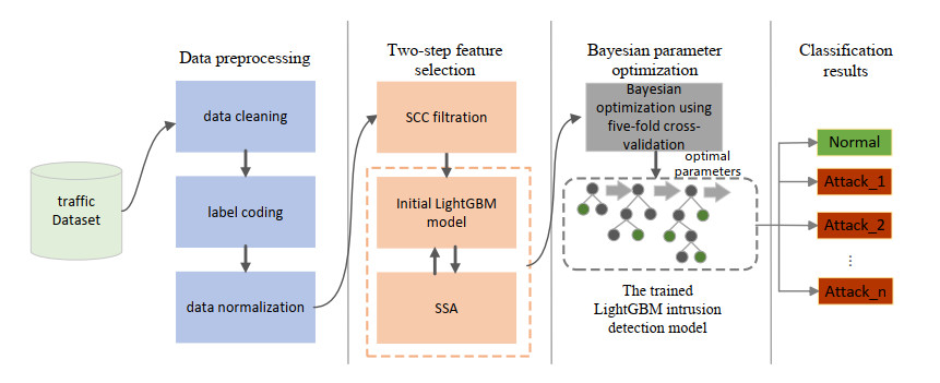
With the widespread application of the Internet of Things (IoT), security risks are becoming increasingly severe. However, due to the limitations in computing resources and energy consumption of IoT devices, traditional intrusion detection models are difficult to apply directly. Although existing methods offer high detection rates, they generally suffer from issues such as complex model structures and deployment difficulties. To address these problems, a lightweight intrusion detection method based on two-stage feature selection and Bayesian optimization is proposed. The method first employs the Spearman Correlation Coefficient (SCC) for filter-based selection to remove redundant features. Then, the Salp Swarm Algorithm (SSA) is used for wrapper-based selection to obtain the optimal feature subset. Finally, a lightweight and efficient LightGBM classifier is constructed, with its parameters adaptively optimized using Bayesian optimization. Unlike previous LightGBM-based IDS studies that rely on manually pruned features and heuristic parameter tuning, this work is the first to couple an SCC–SSA two-stage selection pipeline with Bayesian optimization, providing a fully automated and resource-aware workflow tailored for IoT devices. Experimental results show that the proposed method achieves classification accuracies of 97.22% and 96.08% on the TON_IoT and UNSW-NB15 datasets, respectively. Among them, the model size on the UNSW-NB15 dataset is only 1.77 MB, fully demonstrating its excellent detection performance and lightweight characteristics, making it suitable for deployment on resource-constrained IoT terminal devices.

Keywords:

Citation: Dainan Zhang, Dehui Huang, Yanying Chen, Songquan Lin, Chuxuan Li. A lightweight IoT intrusion detection method based on two-stage feature selection and Bayesian optimization[J]. AIMS Electronics and Electrical Engineering, 2025, 9(3): 359-389. doi: 10.3934/electreng.2025017

Related Papers:

[1]	B Naresh Kumar, Jai Sukh Paul Singh . Intelligence-based optimized cognitive radio routing for medical data transmission using IoT. AIMS Electronics and Electrical Engineering, 2022, 6(3): 223-246. doi: 10.3934/electreng.2022014
[2]	Efe Francis Orumwense, Khaled Abo-Al-Ez . Internet of Things for smart energy systems: A review on its applications, challenges and future trends. AIMS Electronics and Electrical Engineering, 2023, 7(1): 50-74. doi: 10.3934/electreng.2023004
[3]	Abdullah Yahya Abdullah Amer, Tamanna Siddiqu . A novel algorithm for sarcasm detection using supervised machine learning approach. AIMS Electronics and Electrical Engineering, 2022, 6(4): 345-369. doi: 10.3934/electreng.2022021
[4]	Abdul Yussif Seidu, Elvis Twumasi, Emmanuel Assuming Frimpong . Hybrid optimized artificial neural network using Latin hypercube sampling and Bayesian optimization for detection, classification and location of faults in transmission lines. AIMS Electronics and Electrical Engineering, 2024, 8(4): 508-541. doi: 10.3934/electreng.2024024
[5]	Zaineb M. Alhakeem, Heba Hakim, Ola A. Hasan, Asif Ali Laghari, Awais Khan Jumani, Mohammed Nabil Jasm . Prediction of diabetic patients in Iraq using binary dragonfly algorithm with long-short term memory neural network. AIMS Electronics and Electrical Engineering, 2023, 7(3): 217-230. doi: 10.3934/electreng.2023013
[6]	Mostafa A.R. Eltokhy, Mohamed Abdel-Hady, Ayman Haggag, Hisham A. Hamad, Tarek Hosny, Ahmed A. F. Youssef, Ali M. El-Rifaie . An indoor IoT-based LiFi system using LEDs for sensor data transfer. AIMS Electronics and Electrical Engineering, 2025, 9(2): 118-138. doi: 10.3934/electreng.2025007
[7]	Fuhong Meng, Guowu Yuan, Hao Zhou, Hao Wu, Yi Ma . Improved MViTv2-T model for insulator defect detection. AIMS Electronics and Electrical Engineering, 2025, 9(1): 1-25. doi: 10.3934/electreng.2025001
[8]	K.V. Dhana Lakshmi, P.K. Panigrahi, Ravi kumar Goli . Machine learning assessment of IoT managed microgrid protection in existence of SVC using wavelet methodology. AIMS Electronics and Electrical Engineering, 2022, 6(4): 370-384. doi: 10.3934/electreng.2022022
[9]	Lawrence O. Aghenta, M. Tariq Iqbal . Design and implementation of a low-cost, open source IoT-based SCADA system using ESP32 with OLED, ThingsBoard and MQTT protocol. AIMS Electronics and Electrical Engineering, 2020, 4(1): 57-86. doi: 10.3934/ElectrEng.2020.1.57
[10]	Cherechi Ndukwe, M. Tariq Iqbal, Xiaodong Liang, Jahangir Khan, Lawrence Aghenta . LoRa-based communication system for data transfer in microgrids. AIMS Electronics and Electrical Engineering, 2020, 4(3): 303-325. doi: 10.3934/ElectrEng.2020.3.303

Abstract

1. Introduction

For the last couple of years, the evolution of related technologies such as 5G communication, cloud computing, and artificial intelligence has made the application of the Internet of Things (IoT) increasingly widespread, and gradually derived new network application scenarios such as smart cities ^[1], smart healthcare, smart grids, and industrial IoT ^[2,3]. The application of IoT technology enhanced work efficiency and quality of life and optimized resource management. In general, the development of the Internet of Everything has made life more convenient and efficient. However, with the continuous appearance of new technologies, network security issues have become increasingly prominent. Therefore, there is an immediate need for a complete and stable system to ensure the security of the IoT ^[4,5].

IoT is a network that extends from the Internet. It realizes data exchange, communication, and control by connecting various physical devices and objects to the Internet. Due to the huge amount of IoT devices exposed to the Internet, this makes the structure of the IoT more complex and thus more vulnerable to many security threats ^[6,7]. Therefore, to ensure the sustainable development of the IoT and maintain the security of related IoT scenarios, it is necessary to study intrusion detection solutions for IoT environments. An intrusion detection system (IDS) is a security device designed to monitor a network or system for unusual activity ^[8]. It is classified as misuse-based IDS and anomaly-based IDS according to the detection method. Misuse-based IDS identifies attacks based on the matching of data patterns with the records in a signature database. The defect is that it can only identify known types of attacks. Anomaly-based IDS identifies malicious behavior where user behavioral activity deviates from normal operation, with the main advantage of detecting zero-day attacks ^[9,10,11].

In IoT intrusion detection research, machine learning has become the mainstream research strategy because of its strong self-learning ability and generalization performance. However, because IoT networks are usually deployed on resource-constrained devices and have domain-specific traffic characteristics, traditional models cannot be applied directly ^[12,13,14]. Consequently, researchers have proposed lightweight approaches ^[15,16]. But these model schemes generally present some problems, such as excessive pursuit of detection rate, which leads to a low lightweight degree of the model. Although these models have been more streamlined than traditional complex model schemes, they still fail to meet the lightweight detection requirements, and most studies have not fully verified the lightweight degree of their models.

In this paper, we propose a lightweight intrusion detection method based on two-stage feature selection and Bayesian optimization LightGBM, which can be directly applied to intrusion detection of IoT devices. The lightweight of IDS is realized from data and model levels. First, at the data level, a two-stage feature selection combining filtered and wrapped approaches is used to filter the best subset of features in order to reduce the complexity and improve the interpretability of the traffic detection model. Secondly, at the model level, LightGBM with a higher lightweight degree is used as the intrusion detection model. It has the benefits of higher accuracy, smaller memory footprint, and faster training and prediction compared to other models, and can be better applied to IoT devices. In addition, to optimize the detection model, a Bayesian optimization algorithm (BOA) is introduced to improve the parameter optimization efficiency. The primary contributions of this paper are summarized below.

(1) The two-stage feature selection method is proposed to filter the best subset of features. First, we use SCC-based filtered feature selection to select the original features that need to be input, and then use the SSA-based wrapped feature selection method to filter the best feature subset.

(2) To speed up the training of the intrusion detection model and obtain better model performance, a lightweight gradient boosting tree model based on Bayesian optimization LightGBM is proposed.

(3) Finally, the lightweight degree of the LightGBM model and the other four models are tested. Experiments using the UNSW-NB15 and TON_IoT datasets validate that the proposed model is superior to the comparison models in both detection performance and lightweight.

The remainder of this paper is organized as follows: Section 2 introduces recent research on intrusion detection. Section 3 describes the proposed lightweight intrusion detection method. In Section 4, we test the performance of the model and the degree of lightness through experimental results. Finally, Section 5 makes a comprehensive analysis and summary of the paper.

2. Related works

2.1. Deep-learning-based IDS

In this section, we investigate the research on intrusion detection for IoT, most of which is mainly deep learning (DL) based. Imrana et al. ^[17] proposed a bidirectional Long-Short-Term-Memory (BiDLSTM)-based Recurrent Neural Network (RNN) model for detecting attacks in the network. The experimental results on the NSL-KDD dataset demonstrate that the detection performance of the BiDLSTM model outperforms that of traditional LSTM and other advanced models. Yang et al. ^[18] proposed a distributed system based on BiDLSTM and attention method to detect fog nodes in IoT applications, and achieved an accuracy of 99.05% on the UNSW-NB15 dataset. Zarai et al. ^[19] developed an IDS based on RNN and Deep Neural Network (DNN). The author compared the performance of the algorithm with Naive Bayes, Decision Tree, and Support Vector Machine (SVM) and proved that the algorithm was superior to other algorithms. Diro and Chilamkurti ^[20] applied ML to attack detection in IoT and experimentally showed that deep models are more effective than shallow models in attack detection. To make IDS better adapt to the elaborate network environment of the IoT, Zhang et al. ^[21] investigated a model based on an improved Genetic Algorithm (GA) and Deep Belief Network (DBN). They used the GA to optimize the number of hidden layers and neurons in each layer of the neural network in DBN, which effectively improved the detection rate of the attack types.

2.2. Feature-engineering and hybrid optimization

In the Internet of Things environment, IDS usually face challenges such as large data size, high feature dimensions, and limited computing resources. Traditional IDS mostly relies on machine learning (ML) or deep learning algorithms to build models, focusing on the improvement of detection accuracy, but less on optimizing data structures from the feature dimension. With the increasing number of devices and communication frequency, the original data often contains a large number of redundant, irrelevant, and even noisy features, which seriously affects the training efficiency and reasoning performance of the model. Therefore, the introduction of efficient feature engineering and optimization strategies not only helps to reduce the computational burden but also significantly improves detection speed and accuracy, which has become one of the key directions of current research.

In order to solve these problems, Choi et al. ^[22] studied a new method for deep feature extraction and selection (D-FES), which combines stacking feature extraction with weighted feature selection. The practicability of D-FES was proved by experiments, which achieved an accuracy of 99.918% and decreased the false alarm rate to 0.012%. Kim et al. ^[23] used a feature selection method to filter the optimal subset containing a few features to achieve the dimensionality reduction effect to deal with the high dimensionality issue of massive data. To address the issues of input data redundancy and irrelevant features, Vijayanand et al. ^[24] designed an IDS based on the hybrid feature technology of GA and mutual information (MI). Gupta et al. ^[25] proposed a network attack detection system based on a hybrid feature dimension reduction method. They applied NSL-KDD and two IoT dataset experiments to confirm the performance of the proposed framework relative to existing detection frameworks. Alhakami et al. ^[26] developed a new nonparametric Bayesian-based IDS method to study the anomaly-based intrusion detection problem. It differs from classical clustering methods in that specifying the clustering number is not necessary, and the method is capable of addressing issues related to overfitting and underfitting. Qureshi et al. ^[27] aimed to efficiently and quickly train the model by removing, reducing, and selecting meaningless and zero-valued features from the dataset, to get preferable accuracy during model training. Oreški et al. ^[28] conducted feature selection through two stages: feature extraction and feature selection. In the first stage, feature extraction is performed using the Principal Component Analysis (PCA) algorithm. In the second phase, four methods are used for feature selection and ultimately for feature reduction. Yousaf et al. ^[29] proposed using the energy vector derived from DWT-Multiresolution Analysis (MRA) and Parseval's Theorem as input for the ANN, and leveraging Bayesian Optimization to automatically search for hyperparameters such as the number of network layers and learning rate. In 2022, Yousaf et al. ^[30] proposed the 2-ms voltage transients extracted by DWT to input into a tuned Bi-LSTM + Attention model, which maintained an accuracy of 98.6% under high noise (20–45 dB) and resistances of 10–400 $\Omega$ . In a follow-up study, Yousaf et al. ^[31] embedded a wavelet-energy feature extractor and a Bayesian-optimized feed-forward neural network directly inside a DSP-based sensor, cutting the mean location error to 0.514% of the line length.

2.3. Lightweight IDS for edge/IoT devices

With the large-scale deployment of IoT devices, network intrusion detection tasks are gradually shifting from the cloud to the edge for real-time processing. However, edge/IoT devices usually have the characteristics of weak computing power, small storage space, and limited power consumption, which poses a serious challenge to traditional IDS based on complex deep learning structures. In this context, the design of a lightweight IDS model with both high detection performance and resource efficiency has become a research hotspot.

Aiming at the intrusion detection requirements of IoT devices, Zhao et al. ^[32] proposed a lightweight IDS combining convolutional neural networks (CNN) and LightGBM. The author carried out multi-classification experiments on two IoT datasets. Compared with other models, it was proved that the model had better detection ability and lightweight characteristics. Similarly, Yao et al. ^[33] also used the LightGBM model to apply it to edge industrial IoT hybrid intrusion detection and perform lightweight analysis on IoT devices. The study proved that the LightGBM model has the highest accuracy and the lowest training time compared with other comparison models. Okey et al. ^[34] proposed an IDS based on optimized CNN, developed a novel ensemble model for lightweight transfer learning, and achieved good results in image classification. Lahasan et al. ^[35] studied a lightweight autoencoder depth model with a two-layer optimizer. Based on the experimental results obtained from the N-baiot dataset, it has been proven that the optimization model overcomes other models. Similarly, Basati et al. ^[36] proposed a lightweight structure based on a parallel deep autoencoder. The structure uses extended and traditional convolution filters to capture the local and surrounding information of a single parameter in the feature vector, thereby increasing the detection performance of the model. Altaf et al. ^[37] studied a NIDS framework based on a graph neural network (GNN), which makes the model more lightweight and improves the attack rate of detection. Jan et al. ^[38] investigated a lightweight IoT anomaly detection intrusion system using a SVM-based algorithm. The lightweight of the proposed algorithm is demonstrated by experiments.

Based on the above research, it can be seen that most researchers use ML or DL methods to construct IoT intrusion detection research programs. Although these schemes have achieved high detection results on relevant benchmark datasets, most studies lack attention to the degree of model lightweight, or the degree of model lightweight is low, which makes the proposed model more complex and difficult to apply to resource-constrained IoT devices. The summary of the above literature is shown in Table 14 and Table 15 in the Appendix.

3. Proposed methodology

To address the problem of a low degree of lightweight model, we propose a lightweight intrusion detection model based on two-stage feature selection and Bayesian optimization LightGBM. This section introduces in detail the LightGBM algorithm, two-stage feature selection method, and BOA used in the model.

3.1. Lightweight intrusion detection model

The specific process of constructing a lightweight IDS based on two-stage feature selection and Bayesian optimization LightGBM is shown in Figure 1 and includes three stages: data preprocessing, two-stage feature selection, and Bayesian parameter optimization. In order to further clarify the integrity and operability of the proposed framework, this paper provides an end-to-end lightweight intrusion detection system algorithm in Appendix 4. The specific contents of each part are as follows:

Figure 1. Lightweight intrusion detection model architecture.

DownLoad: Full-Size Img PowerPoint

(1) The data preprocessing stage is responsible for the preliminary preprocessing of the collected traffic dataset, so as to facilitate the subsequent introduction of LightGBM for training. Specifically, this stage consists of three elements: data cleaning, label coding, and data normalization. Data cleaning is responsible for removing duplicates and outlier samples from incoming datasets. Label coding is responsible for encoding character-based features in the dataset into numerical features that can be recognized by the model. Finally, data normalization is responsible for scaling the data between $[0, 1]$ to eliminate the dimensional differences between different features. The normalization function uses Equation (3.1).

$\begin{equation} \stackrel{-}{x }\: = \frac{{x - {x_{\min }}}}{{{x_{\max }} - {x_{\min }}}}. \end{equation}$

(3.1)

(2) The two-stage feature selection phase is used to filter the optimal feature subset by combining filtered and wrapped feature selection methods. The preprocessed dataset will first perform SCC-based filtered feature selection to eliminate irrelevant or weakly correlated features. Then, the preliminary reduced dataset is searched for the final feature subset by SSA-based wrapper feature selection. The LightGBM model in the wrapper feature selection uses initial parameters.

(3) The Bayesian parameter optimization stage uses a BOA to achieve fast optimization of LightGBM model parameters. The optimization process uses the average F1 value of LightGBM five-fold cross-validation as the output of the model, and different model parameter combinations as input. After obtaining the optimal parameters, the LightGBM model is trained using all datasets. Finally, classification results are output.

3.2. Two-stage feature selection method

Feature selection aims to screen the best subset of features that can significantly classify abnormal traffic, so as to eliminate redundant and irrelevant features and improve the efficiency and interpretability of the detection model. We use a two-stage feature selection method based on filtering and wrapping to select the optimal feature subset. First, the input original features will use SCC-based filtering feature selection. The role of this step is to eliminate irrelevant or weakly related features to reduce the feature search space for subsequent wrapper selection. Then, an SSA-based wrapping feature selection algorithm is utilized to search for the subset of features that makes the model detection performance optimal.

3.2.1. Filtering feature selection based on SCC

Pearson correlation coefficient (PCC), Spearman correlation coefficient (SCC), and Kendall correlation coefficient (KCC) are three common measures of feature correlation. Generally, PCC is used to measure the linear relationship between two variables, but it is sensitive to outliers and requires data to approximate normal distribution. The KCC is mainly used to judge the consistency between ordered categorical variables, and the computational complexity is relatively high, which is not suitable for large-scale data. In contrast, the SCC used in this paper is based on the rank relationship of variables, which can capture the nonlinear monotonic relationship, is more robust to outliers, and has higher computational efficiency. Therefore, it is more suitable for datasets with high feature dimensions and complex distribution such as Internet of Things traffic data.

The definition of SCC is shown in Equation (3.2).

$\begin{equation} \rho = 1 - \frac{{6\sum\limits_{i = 1}^n {d_i^2} }}{{n({n^2} - 1)}}. \end{equation}$

(3.2)

Where $d_i$ is the rank difference between the two eigenvalues, "rank" is the location of the sorted eigenvalues, and $n$ represents the number of features. The larger the correlation coefficient, the stronger the relationship between each two features and vice versa.

The SCC-based filtered feature selection algorithm is shown in Algorithm 1 in appendix.

3.2.2. Salp Swarm Algorithm

The Salp Swarm Algorithm (SSA) ^[39] is a new swarm intelligence optimization algorithm proposed by Mirjalili et al. ^[40] in 2017. This algorithm is inspired by the chain movement and foraging swarming behavior of salp. In order to adapt to the optimization issues, the SSA defines the salp swarm as two populations: leader and follower. The leader salp is located at the beginning of the chain, and the other salps are the followers. The specific mathematical model is shown below.

It is assumed that the search space of the population is the Euclidean space of $G \times N$ , $G$ is the spatial dimension, and $N$ is the population size. ${X_{\rm{n}}} = {\left[{{X_{n1}}, {X_{n2}}, \cdots {X_{nG}}} \right]^T}$ is used to represent the position of each individual in the space, and ${F_{\rm{n}}} = {\left[{{F_{n1}}, {F_{n2}}, \cdots {F_{nG}}} \right]^T}$ represents the position of the food, where $n = 1, 2, ..., N$ . Therefore, the population initialization expression is

$\begin{equation} {X_{G \times N}} = rand(G, N).\left( {UB - LB} \right) + LB. \end{equation}$

(3.3)

The update of the leader 's position is only related to the relative position of the food, so the update of the leader 's position is denoted as

$\begin{equation} {X_{1, {\rm{g}}}} = \left\{ {\begin{array}{*{20}{c}} {{F_g} + {C_1}\left[ {\left( {UB - LB} \right){C_2} + LB} \right]}&{{C_3} \ge 0.5}\\ {{F_g} - {C_1}\left[ {\left( {UB - LB} \right){C_2} + LB} \right]}&{{C_3} < 0.5} \end{array}} \right.. \end{equation}$

(3.4)

where $X_{1, g}$ and $F_g$ are the positions of the leader and the food in the g-dimensional space, respectively, and UB and LB are the upper and lower bounds of the search space, respectively. $C_2^{\prime }$ and $C_3^{\prime }$ are random numbers between $[0, 1]$ , $C_1^{\prime }$ convergence factor, and the expression is

$\begin{equation} C_1^{\prime } = 2{e^{ - (4\text{t}/T)^2}}. \end{equation}$

(3.5)

In the formula, $t$ is the current number of iterations, and $T$ is the maximum number of iterations.

The position update formula of salp followers is

$\begin{equation} X_{i, g}^{\prime } = \frac{{{X_{i, g}} + {X_{i - 1, g}}}}{2}. \end{equation}$

(3.6)

Where $X_{i, g}^{\prime }$ and ${X_{i, g}}$ are the positions of followers after and before the g-dimensional update, respectively.

3.2.3. Wrapping feature selection based on SSA

The process of searching for the best subset of features is an NP-hard issue ^[41]. Traditional search strategies such as forward search and backward elimination are based on simple greedy heuristic methods to select or discard features, without considering the dependence between features from a global perspective. Therefore, it makes the selected feature subsets local optimal solutions. To solve this problem, a meta-heuristic algorithm SSA is used as a search strategy for wrapper feature selection. SSA has good global exploration and local optimization ability and can search the optimal feature subset from a global perspective. After the first step of filtering selection, the search space is further reduced so that it is easier for the algorithm to obtain the optimal solution.

In order to adapt to the feature selection problem, we set the upper and lower bounds of the SSA search in the range of 0 to 1 and apply binary coding to the fitness function. 0 and 1 are used to represent the unapplied and applied features, respectively. The specific formula is as follows:

$\begin{equation} {X_{i, g}} = \left\{ {\begin{array}{*{20}{c}} 1&{{X_{i, g}} > 0.5}\\ 0&{{X_{i, g}} \le 0.5} \end{array}} \right.. \end{equation}$

(3.7)

The SSA-based wrapper feature selection algorithm is shown in Algorithm 2 in appendix.

In Algorithm 2, the fitness function of the SSA algorithm uses the average F1 value of stratified five-fold cross-validation. Compared with accuracy, the F1-score can better evaluate the model classification performance under unbalanced datasets.

3.3. Bayesian optimization algorithm

The model parameters have a large impact on the performance of the detection model. When establishing the LightGBM detection model to detect abnormal traffic, in order to realize the fast and efficient parameter optimization process, we introduce the BOA to optimize the model parameters.

Bayesian optimization is a global optimization algorithm, which is suitable for solving the black box problem with an unknown derivative of the objective function and a high cost of evaluating the objective function ^[42]. The core of the algorithm is to model the objective function through a probabilistic surrogate model, and then continuously collect new evaluation points near the points that may be the optimal values or unsampled areas to update the surrogate model. This way, the surrogate model approximates the real objective function and then searches for the optimal solution. Among them, the determination of new evaluation points is a typical problem of balancing exploration and development. BOA measures the benefits of new evaluation points for optimization by constructing an acquisition function and determines new evaluation points by maximizing the acquisition function. The specific algorithm steps of Bayesian optimization are shown in Algorithm 3 in appendix.

The probabilistic surrogate model and optimization strategy are the two main components of BOA. The probabilistic surrogate model not only provides an estimate of the objective function, but also provides uncertain information related to the estimate. Common surrogate models include the Gaussian process, Random Forest (RF), and DNN. The optimization strategy usually uses the acquisition function to define the position of the next sampling point. The acquisition function is generally pushed by the surrogate model, and the goal is to maximize the optimal solution. In this paper, the Gaussian process and the simple and easy-to-use Probability of Improvement (PI) function are used as the probability proxy model and the acquisition function, respectively.

3.4. Light Gradient Boosting Machine

Light Gradient Boosting Machine (LightGBM) is a tree-based model with the advantage of efficient feature splitting^[43]. It is an optimization and enhancement of the classical Gradient Boosting Decision Tree (GBDT) algorithm ^[44]. It improves the problem of GBDT in space consumption and time overhead and reduces the training time without reducing the prediction accuracy, thus greatly reducing memory usage. Experiments on the Higgs dataset show that LightGBM is nearly $10$ times faster than the Extreme Gradient Boosting (XGBoost) algorithm, which is also based on an improved GBDT algorithm, and the memory occupancy rate is about $1/6$ of XGBoost. LightGBM mainly adopts the following four aspects to improve its lightweight degree.

3.4.1. Histogram algorithm

The histogram algorithm is the basis and core of the LightGBM algorithm. It is a commonly used algorithm for statistical data distribution. As can be seen from , its basic process is to divide the eigenvalues of each feature into several intervals according to a certain binning method, and then calculate the number of samples and the mean of the target variable in each interval. Finally, the statistical information is stored in a histogram. In the training process, when selecting an optimal splitting point each time, the information gain from each candidate splitting point can be quickly calculated by the statistical information of the histogram, thereby quickly finding the optimal split point. The histogram algorithm does not need to store the results of feature pre-ordering, and can only save the values after feature discretization. These values are enough to be stored with only 8-bit integer variables, which means that the memory consumption can be greatly reduced and only accounts for $1/8$ of the original memory. In addition, when calculating the splitting gain of a node in the decision tree, the histogram-based algorithm uses only $k$ calculations, thus reducing the time complexity of node splitting from $O(\#data*\#feature)$ to $O(k*feature)$ , where $k$ is the number of feature intervals and $\#data > > k$ ..

Figure 2. Histogram algorithm.

DownLoad: Full-Size Img PowerPoint

In addition to using the histogram algorithm to store and split features, LightGBM also uses histogram difference acceleration to further optimize the tree-building process. As shown in , the histogram of a leaf node can be constructed by subtracting the histogram of the parent node from its neighboring nodes, which doubles the speed of the algorithm. In general, constructing a histogram requires going through each data of a leaf node, but using a histogram for subtraction only requires going through $k$ bins of the histogram. In addition, the LightGBM algorithm can first compute the leaf nodes with small histograms and then use the histograms to do the subtraction operation to obtain the leaf nodes with large histograms ^[45]. This effectively avoids repeated computations, reduces memory usage, and improves the scalability of the algorithm. It is particularly suitable for processing large datasets.

Figure 3. Histogram difference process.

DownLoad: Full-Size Img PowerPoint

3.4.2. Leaf-wise strategy with depth constraints

Based on the histogram algorithm, LightGBM is further optimized. It does not use the level-wise growth strategy of most GBDT algorithms, but uses the leaf-wise growth algorithm with depth constraints, as shown in Figure 4 and Figure 5. The leaf-wise growth strategy is to search for the leaf with the largest splitting gain among all the leaves each time and split it until a preset condition is reached. With the same number of divisions, leaf-wise growth produces less error than level-wise growth. However, leaf-wise growth with constant splitting of only one leaf per layer may lead to model overfitting. Therefore, LightGBM limits the depth of the tree during leaf-wise growth to prevent overfitting.

Figure 4. Level-wise tree growth.

DownLoad: Full-Size Img PowerPoint

Figure 5. Leaf-wise tree growth.

DownLoad: Full-Size Img PowerPoint

3.4.3. Gradient-based One-Side Sampling (GOSS)

In GBDT, the gradient value of the sample is related to the learning degree of the sample. The magnitude of the gradient reflects the weight of the sample, with a smaller gradient indicating a better model fit. For these small gradient samples, the simple approach is to discard them directly. However, this will change the distribution of data, which in turn affects the performance of the training model. So as to avoid this issue, LightGBM proposes the new sample sampling algorithm GOSS.

The GOSS algorithm chooses to leave samples with larger gradients and randomly selects samples with smaller gradients. To counteract the effect of random sampling on the distribution of the data, when calculating the information gain, GOSS introduces a constant factor for small gradients. GOSS first sorts the samples according to the absolute value of the gradient and selects the top $m\times100\%$ of the samples. Then, a random sample of $n\times100\%$ is taken from the rest of the data, and this $n\times100\%$ of the small gradient sampled data is multiplied by a constant $(1-m)/n$ for the calculation. This approach reduces the number of data points that have to be taken into account during the construction of histograms and tree growth, making the model training more focused on under-trained samples without changing the distribution of the original dataset too much. The specific relationship of sampling is shown in Figure 6.

Figure 6. GOSS process.

DownLoad: Full-Size Img PowerPoint

3.4.4. Exclusive Feature Bundling (EFB)

EFB is used to reduce the number of features. High-dimensional data tends to be sparse, and this sparsity of the feature space opens up the possibility of lossless merging of features. In order not to lose feature information, mutually exclusive features are usually bundled together. For features that are partially, not completely, mutually exclusive, as long as the degree of non-mutual exclusion between features is less than the conflict ratio defined by EFB, EFB also considers them to be mutually exclusive and bundles them. Because EFB tolerates a small number of conflicts between features, it can obtain fewer features to further improve computational efficiency.

In addition, by fusing and bundling mutually exclusive features, EFP reduces the number of features while also changing the time complexity of constructing histograms from $O(\#data*\#feature)$ to $O(\#data*\#bundle)$ , and $\#bundle < < \#feature$ , thus greatly accelerating the training speed of GBDT. Therefore, EFB further improves the efficiency of the histogram algorithm while reducing the number of features, and accelerating the growth of the leaf-wise tree.

4. Experiment and result analysis

4.1. Hardware and software environment

The simulation environment includes hardware with Intel(R) Core(TM) i3-10100 CPU @ 3.60GHz processor, 8G memory. The software includes Windows10 operating system, Python3.9.0, Anaconda3, Jupyter notebook, scikit-learn1.1.3, CatBoost1.0.0, and lightgbm3.3.2.

4.2. Benchmark datasets

4.2.1. TON_IoT dataset

The experiment in this chapter uses the TON_IoT ^[46] network traffic dataset created based on the real IoT environment. The dataset contains 43 feature attributes and 9 attack types. In order to avoid model overfitting, we have eliminated the timestamp, source and destination IP, and source and destination port attributes, as suggested by the original authors. Table 3 shows the distribution of specific label types in the TON_IoT dataset.

4.2.2. UNSW-NB15 dataset

To examine the detection rate and generalization ability of the IDS proposed by this paper, comparative validation is carried out using the UNSW-NB15 dataset. The UNSW-NB15 ^[47,48] dataset was collected and organized by researchers at the University of New South Wales in 2015 to provide real-world scenario data for modern cybersecurity attacks. The dataset contains 42 features and 9 different types of attacks. Table 1 shows the distribution of specific label types in the UNSW-NB15 dataset.

Table 1. Sample distribution on TON_IoT and UNSW-NB15 datasets.

TON_IoT		UNSW-NB15
Class	Sample size	Class	Sample size
normal	300000	normal	93000
scanning	20000	Generic	58871
password	20000	Exploits	44525
dos	20000	Fuzzers	24246
xss	20000	DoS	16353
backdoor	20000	Reconnaissance	13987
injection	20000	Analysis	2677
ransom ware	20000	Backdoors	2329
ddos	20000	Shellcode	1511
mitm	1043	Worms	174
Total	461043	Total	257673

| Show Table

DownLoad: CSV

4.3. Evaluation indicators

In the IoT scenario, the detection model needs to take into account the classification performance and lightweight degree. Therefore, in this paper, indicators such as accuracy, precision, recall, and F1-score are used to verify the classification performance of the model, and model size, training time, and testing time are used to verify the lightweight degree of the model. Among them, the indicators related to classification performance come from the four basic attributes that describe the confusion matrix, namely true positive (TP), true negative (TN), false positive (FP), and false negative (FN). TP refers to the number of samples that are divided into positive samples and classified correctly. TN refers to the number of samples that are divided into negative samples and classified correctly. FP refers to the number of samples that are divided into positive samples but classified incorrectly. FN refers to the number of samples that are divided into negative samples but classified incorrectly. The specific definitions and calculation methods of each index are as follows.

Accuracy refers to the ratio of the correct classification of the model in all samples.

$Accuracy = \frac{{TP + TN}}{{TP + TN + FP + FN}}$

Precision refers to the accuracy of the model when the predicted sample is positive.

$Precision = \frac{{TP}}{{TP + FP}}$

Recall rate refers to the ability of the model to successfully identify all true positives.

$Recall = \frac{{TP}}{{TP + FN}}$

The F1-score is the harmonic average of precision and recall.

$F1-score = \frac{{2 \cdot \Pr ecision \cdot {\mathop{\rm Re}\nolimits} call}}{{\Pr ecision + {\mathop{\rm Re}\nolimits} call}}$

4.4. Parameter setting

The LightGBM algorithm sets the initial parameters as: n_estimators = 100, max_depth = 10, learning_rate = 0.2, min_data_in_leaf = 20, random_state = 100. Model verification adopts stratified five-fold cross-validation.

4.5. Feature selection

In this paper, a combination of filtering and wrapping feature selection methods is used. First, we calculate the SCC between each feature and the classification label, which measures the monotonic relationship between the variables; its larger absolute value indicates the stronger correlation between the feature and the label. In order to eliminate redundant or weakly correlated features, we set the lower limit threshold of correlation and only retain features that are highly correlated with the label. Due to the lack of uniform standards for SCC thresholds in different scenarios, this paper evaluates the impact of different thresholds on model performance through experiments to determine the optimal value. Figure 7 shows the trend of five-fold cross-validation F1-score of TON_IoT and UNSW-NB15 datasets under different thresholds.

Figure 7. Changes in model classification performance under different threshold conditions.

DownLoad: Full-Size Img PowerPoint

From the left image of Figure 7, it can be found that when the threshold is less than or equal to 0.01788, the F1-score of the model remains basically stable, indicating that the redundant or weak correlation features are mainly eliminated at this stage, which has little effect on the classification effect. When the threshold is further improved, the performance of the model decreases significantly, indicating that some key features are deleted by mistake. Therefore, 0.01788 is selected as the optimal threshold for the TON_IoT dataset. Similarly, the right image in Figure 7 shows that the model performs well when the SCC threshold is less than or equal to 0.03074 in the UNSW-NB15 dataset, and the F1-score also decreases after exceeding this value, indicating that the useful features are over-removed. Therefore, 0.03074 is set as the optimal threshold for this dataset. In summary, the selected two thresholds are located at the critical point of performance change, which can maintain the classification performance to the greatest extent while compressing the feature dimension. Table 2 gives the indexes of the features eliminated by the two datasets under different threshold conditions.

Table 2. Features eliminated by SCC-based filtering feature selection algorithm.

Dataset	Correlation coefficient threshold	Eliminated feature index	Eliminated number
TON_IoT	0.01788	24, 23, 29, 33, 34, 32, 26,	14
		27, 4, 25, 30, 31, 28, 20
UNSW-NB15	0.03074	36, 37, 28, 38, 1	5

| Show Table

DownLoad: CSV

Next, the wrapper feature selection is performed on the filtered features, and the number of populations with $N = 30$ and the number of iterations with $T = 200$ are set. The features selected by the SSA-based wrapper feature selection algorithm for the TON_IoT and UNSW-NB15 datasets are listed in Table 3.

Table 3. Features selected by SSA-based wrapper feature selection algorithm.

TON_IoT		UNSW-NB15
Feature index	Feature name	Feature index	Feature name
0	proto	2	xServ
3	src_bytes	3	xState
5	conn_state	5	dpkts
6	missed_bytes	6	sbytes
7	src_pkts	7	dbytes
8	src_ip_bytes	9	sttl
10	dst_ip_bytes	12	dload
11	dns_query	14	dloss
14	dns_rcode	17	sjit
15	dns_AA	18	djit
19	ssl_version	24	synack
21	ssl_resumed	26	smean
		32	ct_dst_ltm
		33	ct_src_dport_ltm
		34	ct_dst_sport_ltm
		35	ct_dst_src_ltm
		40	ct_srv_dst

| Show Table

DownLoad: CSV

4.6. Parameter optimization

Based on the selected features, the hyperparameters of the detection model are optimized. The optimization process uses the Bayesian optimization method to automatically find the optimal parameter combination through intelligent search. The number of iterations of Bayesian optimization is set to 50, and the optimization index is the average F1-score of the five-fold cross-validation of the model. The corresponding parameter search space is shown in Table 4. In order to ensure the effectiveness and stability of the parameter optimization process, this paper proposes the following practical strategies:

Table 4. Bayesian optimization parameter search space.

Parameter name	Parameter space
Number of base classifiers (n_estimators)	(80,550)
Learning rate (learning_rate)	(0.01, 0.20)
Maximum depth of tree body length (max_depth)	(5, 20)
Minimum amount of data of leaf nodes (min_data_in_leaf)	(2, 20)

| Show Table

DownLoad: CSV

(1) Define the optimization objective function: select clear and quantifiable optimization indicators. In this paper, the weighted F1-score is used as the objective function to comprehensively measure the detection performance of different categories.

(2) Determine the parameter search space: combined with the characteristics of the model and experimental experience, set a reasonable and representative parameter interval, not only to ensure sufficient search range, but also to avoid the efficiency decline caused by invalid areas.

(3) Setting the number of iterations: The number of iterations of BOA directly affects the tuning results and computational costs. In this paper, 50 iterations are used to balance performance improvement and resource consumption in a reasonable time.

(4) Stochastic control: By fixing random seeds, the reproducibility of the optimization process results is ensured.

(5) Evaluation strategy: According to the task requirements, the appropriate evaluation strategy is selected. In this paper, five-fold cross-validation is used to evaluate each group of parameters to reduce the error caused by the contingency of data division.

4.7. Result and analysis

4.7.1. The influence of feature selection on the detection effect

In this paper, the detection performance and detection efficiency of models using original features, SCC feature selection, and features after two-step feature selection are compared under initial parameters. It can be seen from Figure 8 and Table 5 that after SCC feature selection, the TON_IoT dataset has a small decline compared with the first four indicators of feature selection, while the UNSW-NB15 dataset does not have this situation. We hypothesize that this may be explained by TON_IoT dataset having rich cross-feature, non-monotonic patterns. SCC misjudges these "weak and strong" signals and drops them, leading to a drop in the metric. Looking further after the two-step feature selection, the TON_IoT dataset achieves better classification performance than all features, while retaining only 12 feature attributes. The accuracy, precision, recall, and F1-score reach 97.04%, 97.58%, 97.04%, and 97.19%, respectively, which are 0.71%, 0.05%, 0.71%, and 0.47% higher than those before feature selection. Similarly, the UNSW-NB15 dataset has better classification performance in SCC feature selection and two-step feature selection than before feature selection, and the accuracy, precision, recall and F1-score reach 94.88%, 94.94%, 94.88%, and 94.81%, respectively. In addition, in terms of detection efficiency, both datasets after feature selection have a certain reduction in the average training and detection time for model cross-validation. Compared with the original features, the training time of TON IoT dataset is reduced by 22.5%, and the time required for traffic detection is reduced by 14.4%.

Figure 8. Comparison of model detection performance before and after feature selection.

DownLoad: Full-Size Img PowerPoint

Table 5. Comparison of model detection efficiency before and after feature selection.

Datasets	Feature selection algorithms	Feature number	Training time	Testing time
TON_IoT	N/A	38	11.23	0.96
	Two-stage feature selection	12	10.48	0.85
UNSW-NB15	N/A	42	0.40	0.03
	Two-stage feature selection	22	0.27	0.03

| Show Table

DownLoad: CSV

4.7.2. Comparison of the proposed method with other feature dimensionality reduction algorithms

In order to further test the superiority of the proposed feature selection method, this paper compares the proposed two-stage feature selection method with three classical feature dimension reduction algorithms: PCA, Recursive Feature Elimination (RFE), and Maximal Information Coefficient (MIC). These three algorithms are used to reduce the original traffic features to the same feature dimension as the two-stage feature selection. The detection indicators of the initial parameter model under different feature dimension reduction methods are shown in Figure 9.

Figure 9. Comparison of feature dimension reduction methods.

DownLoad: Full-Size Img PowerPoint

Combining the results of the left figures in Figure 8 and Figure 9, it can be found that, except for the PCA feature dimension reduction method, the other three methods all show a certain improvement in the performance of the model using the TON_IoT dataset detection. Among them, the proposed two-stage feature selection method has the most obvious improvement. Compared with the best-performing MIC algorithm, the proposed method improves the accuracy, precision, recall, and F1-score by 0.69%, 0.02%, 0.69%, and 0.45%, respectively. Combining the right figures in Figure 8 and Figure 9, the model trained using the UNSW-NB15 dataset only has the detection performance of the model improved by the method proposed in this paper, and the other three dimensionality reduction algorithms have no effect on improving the detection performance of the model.

In summary, our two-stage feature selection method not only effectively selects the best feature subset for model classification but also improves the detection performance of the model better than several other commonly used feature selection methods. It is suitable for feature screening of traffic data.

4.7.3. Comparison before and after model optimization

In this section, BOA, Particle Swarm Optimization (PSO) ^[49], and GA ^[50] are used to optimize the parameters of the LightGBM detection model, so as to explore the influence of parameter optimization method and parameter optimization results on the detection accuracy of the model. The optimized objective function is set as the average F1 value of the five-fold cross-validation, and the number of iterations is 50 times. The parameter optimization results of the two benchmark datasets under the three optimization methods and the detection performance of the optimized model are shown in Table 6, Table 7, and Figure 10, respectively.

Table 6. LightGBM parameter optimization range and optimization value of TON_IoT dataset.

Parameter	Parameter ranges	BOA	PSO	GA
n_estimators	(80,150)	141	128	137
learning_rate	(0.01, 0.1)	0.042	0.037	0.041
max_depth	(5, 15)	9	12	13
min_data_in_leaf	(2, 20)	19	18	7

| Show Table

DownLoad: CSV

Table 7. LightGBM parameter optimization range and optimization value of UNSW-NB15 dataset.

Parameter	Parameter ranges	BOA	PSO	GA
n_estimators	(350,550)	509	467	478
learning_rate	(0.15, 0.20)	0.153	0.164	0.184
max_depth	(5, 20)	19	10	13
min_data_in_leaf	(2, 20)	10	9	2

| Show Table

DownLoad: CSV

Figure 10. Comparison of parameter optimization methods.

DownLoad: Full-Size Img PowerPoint

As can be seen from Figure 10, all three optimization methods bring some performance improvement to the model, among which the Bayesian optimization improvement is the most obvious. The TON_IoT dataset has reached 97.22%, 97.78%, 97.22%, and 97.39% in accuracy, precision, recall and F1-score, respectively, which are 0.19%, 0.21%, 0.19%, and 0.20% higher than those before optimization. Similarly, the performance of the UNSW-NB15 dataset is also improved, which is 1.27%, 1.19%, 1.27%, and 1.33% higher than that before optimization. Moreover, the performance of the models trained through BOA on both datasets is superior to PSO and GA. In terms of optimization time, Bayesian optimization consumes the least time. The TON_IoT dataset consumes 1990.74 s on 50 iterations of Bayesian optimization, which is about 42.29% of PSO and 52.23% of GA, while the UNSW-NB15 dataset only consumes 491.79 s on Bayesian optimization. It can be seen that BOA is more advantageous than PSO and GA in the parameter optimization of LightGBM, and it can output better parameter combinations in a shorter time.

4.7.4. Comparison of detection performance and lightweight degree between different models

Based on the same feature selection strategy and parameter optimization method, LightGBM is compared with a variety of different detection models, including RF, Multilayer Perceptron (MLP), SVM, and CatBoost. The experiment comprehensively evaluates the generalization ability and resource adaptability of each model in different network environments from multiple dimensions such as classification performance, result stability, computational efficiency, and model lightweight.

Table 8 and Table 9 show the classification results of LightGBM on TON_IoT and UNSW-NB15 datasets. Experiments show that LightGBM is superior to other comparison models in terms of classification performance and stability. On the TON_IoT dataset, its accuracy and F1-score reached 97.22% and 97.39%, respectively, and the standard deviation was small, showing strong robustness. On the UNSW-NB15 dataset, LightGBM also leads with an accuracy of 96.08%. Combining various indicators, LightGBM shows excellent classification accuracy, stability, and adaptability to diverse network traffic, and verifies its effectiveness and advantages as an IoT intrusion detection classifier.

Table 8. Comparison of detection performance between different models of TON_IoT.

Algorithms	Accuracy (%)	Precision (%)	Recall (%)	F1-score (%)
RF	97.14±2.36	97.74±1.18	97.14±2.36	97.32±1.99
MLP	96.87±2.33	97.50±1.08	96.87±2.33	97.06±1.93
SVM	97.02±2.52	97.64±1.24	97.02±2.52	97.21±2.12
CatBoost	97.20±2.36	97.74±1.26	97.20±2.36	97.36±2.03
LightGBM	97.22±2.29	97.78±1.18	97.22±2.29	97.39±1.95

| Show Table

DownLoad: CSV

Table 9. Comparison of detection performance between different models of UNSW-NB15.

Algorithms	Accuracy (%)	Precision (%)	Recall (%)	F1-score (%)
RF	96.08±0.20	96.06±0.20	96.08+0.20	96.06+0.20
MLP	94.94±0.07	94.93±0.08	94.94±0.07	94.93±0.06
SVM	94.88±0.13	94.89±0.14	94.88±0.13	94.83±0.14
CatBoost	95.86±0.18	95.85±0.18	95.86±0.18	95.85±0.18
LightGBM	96.08±0.10	96.07±0.10	96.08±0.10	96.07±0.09

| Show Table

DownLoad: CSV

It can be clearly seen from Table 10 and Table 11 that the computational efficiency and resource consumption of each model on the two datasets are significantly different. LightGBM is superior to other models in terms of training time, test time, and overall running time. On the TON_IoT dataset, the training time of LightGBM is only 7.16 s, which is 77.48% shorter than the RF model with the shortest training time, while its test time and total running time remain at the lowest level. On the UNSW-NB15 dataset, LightGBM also shows extremely high computational efficiency. The training and testing time is only 1.48 s and 0.16 s, respectively, which is significantly faster than other comparison models. In addition, LightGBM also performs well in terms of memory usage and model size, and the required resources are significantly lower than most other models. Especially on the UNSW-NB15 dataset, the model volume is only 1.77 MB, which is much smaller than models such as RF and MLP. The above results show that LightGBM not only has excellent computing speed advantages but also can effectively reduce resource consumption, so it is very suitable for rapid deployment and application in resource-constrained environments.

Table 10. Comparison of model efficiency and lightweight performance on TON_IoT dataset.

Algorithms	Training time (s)	Testing time (s)	Running time (s)	Memory occupancy (MB)	Model size (MB)
RF	31.81	1.95	162.12	277.13	26.10
MLP	11706.11	1.99	82650.65	1247.09	15.70
SVM	5512.73	165.62	32622.30	460.88	5.69
CatBoost	265.99	1.53	1284.35	458.84	5.43
LightGBM	7.16	1.11	49.73	224.34	4.69

| Show Table

DownLoad: CSV

Table 11. Comparison of model efficiency and lightweight performance on UNSW-NB15 dataset.

Algorithms	Training time (s)	Testing time (s)	Running time (s)	Memory occupancy (MB)	Model size (MB)
RF	12.30	0.35	59.61	369.84	83.80
MLP	20326.50	5.71	72435.84	499.91	16.60
SVM	1549.36	60.07	7086.95	345.88	3.41
CatBoost	60.38	0.19	292.40	334.29	3.25
LightGBM	1.48	0.16	8.34	299.79	1.77

| Show Table

DownLoad: CSV

4.7.5. Ablation experiment

In order to deeply evaluate the influence of key modules in the proposed method on model performance and computational efficiency, ablation experiments are carried out on two datasets of TON_IoT and UNSW-NB15. By applying a single module and different combination configurations, the performance of each scheme in classification accuracy, recall, F1-score, training time, and test time is compared, so as to analyze the independent role and synergistic effect of each module in the model.

Table 12 and Table 13 show the performance comparison of different combination modules on the two datasets. The experimental results show that the BOA module contributes significantly to improving the classification accuracy, while SSA and SCC focus more on accelerating the training process and improving the computational efficiency. In multiple combination configurations, the three module combination schemes achieve the best classification performance on both TON_IoT and UNSW-NB15 datasets, while maintaining a low training and testing resource consumption, which fully verifies the effectiveness of each module and the good trade-off between accuracy and computational efficiency of the proposed method.

Table 12. Comparison results of ablation experiments for TON_IoT.

Algorithms	Accuracy (%)	Precision (%)	Recall (%)	F1-score (%)	Training time (s)	Testing time (s)
N/A	96.36	97.53	96.36	96.74	9.37	0.83
SCC	96.29	97.46	96.29	96.67	8.76	0.72
SSA	96.64	96.94	96.64	96.73	7.29	0.76
BOA	96.62	97.78	96.62	96.99	11.57	1.27
SCC+SSA	97.04	97.58	97.04	97.19	7.26	0.71
SCC+BOA	96.59	97.76	96.59	96.97	10.69	1.22
SSA+BOA	96.88	97.19	96.88	96.98	8.63	1.18
SCC+SSA+BOA	97.22	97.78	97.22	97.39	7.16	1.11

| Show Table

DownLoad: CSV

Table 13. Comparison results of ablation experiments for UNSW-NB15.

Algorithms	Accuracy (%)	Precision (%)	Recall (%)	F1-score (%)	Training time (s)	Testing time (s)
N/A	94.72	94.81	94.72	94.64	0.90	0.05
SCC	94.81	94.88	94.81	94.73	0.75	0.05
SSA	94.77	94.85	94.77	94.69	0.60	0.06
BOA	95.87	95.85	95.87	95.85	2.21	0.21
SCC+SSA	94.88	94.94	94.88	94.81	0.48	0.05
SCC+BOA	96.04	96.03	96.04	96.03	2.91	0.19
SSA+BOA	95.92	95.91	95.92	95.90	1.75	0.17
SCC+SSA+BOA	96.08	96.07	96.08	96.07	1.48	0.16

| Show Table

DownLoad: CSV

5. Conclusions

In this paper, aiming at the intrusion detection issue of IoT devices, a two-stage feature selection method based on SCC filtering and SSA wrapping is proposed for dimensionality reduction of high-dimensional data and applied to the LightGBM lightweight model. To verify the performance and lightweight of the proposed method, we apply the TON_IoT and UNSW-NB15 datasets to perform hierarchical five-fold cross-validation experiments on the model. The experimental results demonstrate that the proposed feature selection method clearly promotes the performance of the LightGBM model. At the same time, the proposed method is more lightweight than the comparison model in regards to the lightweight degree. On the TON_IoT dataset, the accuracy and F1-score of the LightGBM model after parameter optimization reached 97.223% and 97.390%, respectively. The size of the LightGBM model is only 1.77 MB after training based on the UNSW-NB15 dataset. Therefore, our proposed IDS is able to be better applied to IoT devices to detect network attacks in IoT.

Although this study has achieved good results in algorithm design and performance evaluation, there is still room for improvement on the application of the model in the actual IoT environment. In future work, we will further optimize the practicability and versatility of the proposed model in the following three aspects:

(1) Edge deployment and resource adaptability improvement: It is planned to deploy the model on edge computing platforms such as Raspberry Pi, and evaluate its reasoning delay, memory footprint, and power consumption performance to verify its real-time performance and deployment feasibility in resource-constrained environments.

(2) Enhance the adaptability of dynamic environment and data heterogeneity: Aiming at the frequent changes of multi-source heterogeneous data and network structure in the Internet of Things, the feature alignment and concept drift detection methods are studied to enhance the robustness and continuous detection ability of the model in a complex dynamic environment.

(3) Construction of cross-domain generalization and continuous learning mechanism: Combining transfer learning, incremental learning, and online updating strategies, the generalization ability of the model in the face of new attack modes and different application scenarios is improved, and the stable deployment of the model in a wide range of IoT environments is realized.

Author contributions

Dainan Zhang: Conceptualization, Methodology, Investigation, Code writing, Writing ‒ original draft; Dehui Huang: Software, Validation, Writing ‒ review and editing; Yanying Chen: Code writing, Validation, Data analysis; Songquan Lin: Investigation, Project administration; Chuxuan Li: Data collection, Visualization. All authors approved the final manuscript.

Use of Generative-AI tools declaration

The authors declare that they have not used Artificial Intelligence (AI) tools in the creation of this article.

Acknowledgments

This work is supported by China Southern Power Grid Technology Project (GDKJXM20230780).

Conflict of interest

The authors declare no conflicts of interest in this paper.

Appendix

Algorithm 1 SCC-based filtered feature selection method
Input: Original feature set $S$ = $\{s_1, s_2, \cdots s_m\}$ , Classification label $l$ , Correlation threshold $\tau$
Output: Filtered feature subset $S'$
1: for $i = 1 \to m$ do
2: The SCC ${\rho }_{i}$ of feature $s_i$ and classification label $l$ was calculated according to Equation (3.2).
3: if ${\rho }_{i}$ $<$ $\tau$ then
4: Eliminate traffic characteristics $s_i$
5: else
6: Retain the traffic characteristics $s_i$
7: end if
8: end for

Algorithm 2 SSA-based wraparound feature selection algorithm
Input: Filtered feature subset $S'$ , Classification label $l$ , Population size $N$ , Maximum number of iterations $T$
Output: optimal feature subset $S^* \leftarrow X_{best}$
1: Initialization population $X_n(n = 1, 2, \cdots, N)$
2: According to Equation (3.7), the population is binarized, which is only used to calculate the fitness function without changing the population position.
3: Calculate fitness functiona $fitness(X_n)$ nd Optimal position of salps $X_{best}$
4: for $t = 1 \to T$ do
5: The population is updated according to Equation (3.4)(3.5)(3.6)
6: Update the position of salp across the parameter space
7: Population binaryzation
8: Calculate the fitness function of the new population and update the optimal position $X_{best}$
9: $t = t+1$
10: end for

Algorithm 3 Bayesian optimization algorithm
Input: Initialize the number of $n_0$ points, Maximum number of iterations $N$ , surrogate model $g(X)$ , acquisition function $\alpha(X\|D)$
Output: Optimal candidate evaluation points $\{X^, Y^\}$
1: Randomly initialize $n_0$ points $X_{init} = \{X_0, X_1, \cdots, X_{n_0-1} \}$
2: Obtain the function value of the initialization point $f(X_{init})$ , Get the initial point set $D_0 = \{X_{init}, f(X_{init})\}$
3: Let $t = n_0$ , $D_{t-1} = D_0$
4: while $t < N$ do
5: The surrogate model $g(X)$ is constructed according to the current point set $D_{t-1}$ .
6: According to the surrogate model $g(X)$ , maximize the acquisition function $\alpha(X\|D_{t-1})$ , and get the next evaluation point: $X_t = arg min\alpha(X\|D_{t-1})$
7: Gets the function value $f(X_t)$ of the evaluation point $X_t$ and adds it to the current set of evaluation points: $D_t = D_{t-1}\cup\{X_t, f(X_t)\}$ , turn line 5
8: end while
Output: Optimal candidate evaluation points: $\{X^, Y^\}$

Algorithm 4 End-to-end lightweight IDS
Input: Original feature set $S = \{ {s_1}, {s_2}, \cdots {s_m}\}$ , Classification label $l$ , Correlation threshold $\tau$ ; SSA parameters: population size $N$ , iterations $T$ ; BOA parameters: initial samples ${n_0}$ , max iterations ${N_B}$ , surrogate model $g(X)$ , acquisition function $\alpha (X\|D)$ ;
Output: Trained LightGBM model $M*$
1: $S' \leftarrow \{ \}$ filtered subset
2: for each feature ${S_i} \in S$ do
3: ${\rho _i} \leftarrow$ Spearman Corr $({S_i}, l)$ Equation (3.2)
4: if ${\rho _i} \ge \tau$ then $S' \leftarrow S' \cup \{ {S_i}\}$
5: end for
6: Initialization population ${X_n}(n = 1, 2, \cdots, N)$
7: Binarised population ${X_{i, g}}{\rm{ > }}0.5 \to 1, else \to 0$ Equation (3.7); compute fitness ${X_n}$
8: Evaluate fitness; set ${X_{best}}$
9: for $t = 1 \to T$ do
10: Update position (Equation (3.4)(3.5)(3.6))
11: Binarised population
12: Re-evaluate fitness; update ${X_{best}}$
13: end for
14: ${S^ * } \leftarrow$ features indicated by ${X_{best}}$
15: Random-init ${n_0}$ piont ${X_{init}}$ ; ${D_0} \leftarrow \{ {X_{init}}, f({X_{init}})\}$
16: while ${t_0} \leftarrow {n_0}$ do
17: Fit surrogate $g$ on ${D_{t - 1}}$
18: ${X_t} \leftarrow \arg \max \alpha (X\|{D_{t - 1}})$
19: ${l_t} \leftarrow f(LightGBM\{ {X_t}\} (S*))$
20: ${D_t} \leftarrow {D_{t - 1}} \cup \{ {X_t}, {l_t}\}$
21: $t \leftarrow t + 1$
22: end while
23: $X$ , $Y \leftarrow best(fitness)$ in $D\{ {N_B}\}$
24: Final training
25: $M* \leftarrow LightGBM(X\}$ trained on full data using features $S$
26: return $M*$

Table 14. Comparison of model detection efficiency before and after feature selection.

References	Method	Highlights	Main Limitations (compared with proposed model)
Imrana et al. ^[17]	BiLSTM traffic-sequence IDS	Captures temporal dependencies	No feature selection; large model, inference latency not reported;
Yang et al. ^[18]	Bi-LSTM + Attention	Attention improves interpretability	GPU training required; edge deployment cost high;
Zarai et al.^[19]	Elman-RNN / GRU / DNN comparison	Systematic cross-family benchmark	slow training;
Diro et al. ^[20]	Distributed CNN-GRUedge IDS	Parallel inference concept	model $>$ 15 MB; hardware demand not quantified;
Zhang et al. ^[21]	GA-selected features + DBN	Evolutionary optimisation + deep model	Old dataset; DBN training time high;
Choi et al. ^[22]	Deep abstract features + weighted selection for Wi-Fi spoofing	Tailored to wireless-layer attacks	Highly domain-specific; hard to generalise to generic IoT traffic;
Kim et al. ^[23]	Multi-algorithm FS for 5G DDoS	5G core-network focus	Static filtering only; no model compression;
Vijayanand et al. ^[24]	GA + Mutual-Information hybrid FS	Early dual-stage selector	No modern ensemblemodel; thresholds manually tuned;
Gupta et al. ^[25]	ReliefF + Gini reduction → Random Forest	Combined dimensionality reduction	model $\approx$ 6 MB; Manual hyper-tuning;
Alhakami et al. ^[26]	Non-parametric Bayesian IDS	Unsupervised capability	Heavy training cost; not lightweight;
Qureshi et al. ^[27]	Heuristic GA rule-based IDS	Intuitive rule learning	Rule explosion; weak generalisation;
Oreški et al. ^[28]	k-means + J48 hybrid mining	Simple combination	Lower detection; no feature compression;
Yousaf et al. ^[29]	Wavelet-energy ANN (Bayes-tuned) dual single-ended relays for meshed HVDC protection	Uses wide-area synchrophasor data and adaptive logic to clear pole-to-pole & pole-to-ground faults.	Relies on high-speed PMU infrastructure; unsuitable for resource-constrained IoT edge nodes; No feature-selection or model-size discussion.

| Show Table

DownLoad: CSV

Table 15. Comparison of model detection efficiency before and after feature selection.

References	Method	Highlights	Main Limitations (compared with proposed model)
Yousaf et al. ^[30]	Deep-learning robust DC-fault protection (BiLSTM +Attention)	Bi-LSTM with attention	model $\approx$ 11 MB; Training requires GPU;
Yousaf et al. ^[31]	Optimised intelligent sensor + UKF observer for DC-fault location	Embeds Unscented Kalman Filter & adaptive gain observer in a dedicated DSP	Needs 25 kHz sampling & custom DSP board ( $\approx$ 8 MB flash).
Zhao et al. ^[32]	Plain LightGBM IoT IDS	Fast ensemble inference	model $\approx$ 4 MB; No feature selection;
Yao et al. ^[33]	Edge IIoT hybrid IDS	Edge deployment perspective	Memory not quantified; manual features;
Okey et al. ^[34]	Transfer-learning CNN IDS	Good cross-domain generalisation	model $>$ 12 MB; GPU needed;
Lahasan et al. ^[35]	Optimised denoising auto-encoder IDS	Strong denoising ability	Long train/ decode time; no compression;
Basati et al. ^[36]	Parallel deep auto-encoder (PDAE)	High detection rate	50 M parameters; unsuitable for endpoints;
Altaf et al. ^[37]	NE-GConv lightweight GCN IDS	Graph model, edge-oriented	model $\approx$ 3 MB; no auto hyper-tuning;
Jan et al. ^[38]	Ultra-light IoT IDS	Low-power focus	Lower detection; no dynamic optimisation;

| Show Table

DownLoad: CSV

References

[1]	Solmaz G, Wu FJ, Cirillo F, Kovacs E, Santana JR, Sánchez L, et al. (2019) Toward understanding crowd mobility in smart cities through the internet of things. IEEE Commun Mag 57: 40–46. https://doi.org/10.1109/MCOM.2019.1800611 doi: 10.1109/MCOM.2019.1800611
[2]	Wang T, Luo H, Jia W, Liu A, Xie M (2019) Mtes: An intelligent trust evaluation scheme in sensor-cloud-enabled industrial internet of things. IEEE T Ind Inform 16: 2054–2062. https://doi.org/10.1109/TII.2019.2930286 doi: 10.1109/TII.2019.2930286
[3]	Brotsis S, Limniotis K, Bendiab G, Kolokotronis N, Shiaeles S (2021). On the suitability of blockchain platforms for IoT applications: Architectures, security, privacy, and performance. Comput Netw 191: 108005. https://doi.org/10.1016/j.comnet.2021.108005 doi: 10.1016/j.comnet.2021.108005
[4]	Hassan WH (2019) Current research on Internet of Things (IoT) security: A survey. Comput Netw 148: 283–294. https://doi.org/10.1016/j.comnet.2018.11.025 doi: 10.1016/j.comnet.2018.11.025
[5]	Anthi E, Williams L, Słowińska M, Theodorakopoulos G, Burnap P (2019) A supervised intrusion detection system for smart home IoT devices. IEEE Internet Things 6: 9042–9053. https://doi.org/10.1109/JIOT.2019.2926365 doi: 10.1109/JIOT.2019.2926365
[6]	Abiodun OI, Abiodun EO, Alawida M, Alkhawaldeh RS, Arshad H (2021) A review on the security of the internet of things: Challenges and solutions. Wireless Pers Commun 119: 2603–2637. https://doi.org/10.1007/s11277-021-08348-9 doi: 10.1007/s11277-021-08348-9
[7]	Popoola SI, Adebisi B, Hammoudeh M, Gui G, Gacanin H (2020) Hybrid deep learning for botnet attack detection in the internet-of-things networks. IEEE Internet Things 8: 4944–4956. https://doi.org/10.1109/JIOT.2020.3034156 doi: 10.1109/JIOT.2020.3034156
[8]	Fenanir S, Semchedine F, Baadache A (2019) A Machine Learning-Based Lightweight Intrusion Detection System for the Internet of Things. Revue D Intelligence Artificielle 33: 203–211. https://doi.org/10.18280/ria.330306 doi: 10.18280/ria.330306
[9]	Radivilova T, Kirichenko L, Alghawli AS, Ilkov A, Tawalbeh M, Zinchenko P (2020) The complex method of intrusion detection based on anomaly detection and misuse detection. In: 2020 IEEE 11th International Conference on Dependable Systems, Services and Technologies (DESSERT), 133–137. https://doi.org/10.1109/DESSERT50317.2020.9125051
[10]	Chou D, Jiang M (2021) A survey on data-driven network intrusion detection. ACM Computing Surveys (CSUR) 54: 1–36. https://doi.org/10.1145/3472753 doi: 10.1145/3472753
[11]	Buczak AL, Guven E (2015) A survey of data mining and machine learning methods for cyber security intrusion detection. IEEE Commun Surv Tut 18: 1153–1176. https://doi.org/10.1109/COMST.2015.2494502 doi: 10.1109/COMST.2015.2494502
[12]	Roy S, Li J, Choi BJ, Bai Y (2022) A lightweight supervised intrusion detection mechanism for IoT networks. Future Generation Computer Systems 127: 276–285. https://doi.org/10.1016/j.future.2021.09.027 doi: 10.1016/j.future.2021.09.027
[13]	Cho HH, Wu HT, Lai CF, Shih TK, Tseng FH (2020) Intelligent charging path planning for IoT network over blockchain-based edge architecture. IEEE Internet Things 8: 2379–2394. https://doi.org/10.1109/JIOT.2020.3027418 doi: 10.1109/JIOT.2020.3027418
[14]	Soe YN, Feng Y, Santosa PI, Hartanto R, Sakurai K (2020) Towards a lightweight detection system for cyber attacks in the IoT environment using corresponding features. Electronics 9: 144. https://doi.org/10.3390/electronics9010144 doi: 10.3390/electronics9010144
[15]	Islam N, Farhin F, Sultana I, Kaiser MS, Rahman MS, Mahmud M, et al. (2021) Towards machine learning based intrusion detection in IoT networks. Comput Mater Contin 69: 1801–1821. https://doi.org/10.32604/cmc.2021.018466 doi: 10.32604/cmc.2021.018466
[16]	Wang Z, Li Z, He D, Chan S (2022) A lightweight approach for network intrusion detection in industrial cyber-physical systems based on knowledge distillation and deep metric learning. Expert Syst Appl 206: 117671. https://doi.org/10.1016/j.eswa.2022.117671 doi: 10.1016/j.eswa.2022.117671
[17]	Imrana Y, Xiang Y, Ali L, Abdul-Rauf Z (2021) A bidirectional LSTM deep learning approach for intrusion detection. Expert Syst Appl 185: 115524. https://doi.org/10.1016/j.eswa.2021.115524 doi: 10.1016/j.eswa.2021.115524
[18]	Yang Y, Tu S, Ali RH, Alasmary H, Waqas M, Amjad MN (2023) Intrusion detection based on bidirectional long short-term memory with attention mechanism. CMC-Computer Material and Continua 74: 801–815. https://doi.org/10.32604/cmc.2023.031907 doi: 10.32604/cmc.2023.031907
[19]	Zarai R, Kachout M, Hazber M, Mahdi M (2020) Recurrent Neural Networks & Deep Neural Networks Based on Intrusion Detection System. Open Access Library Journal 7: 1–11. https://doi.org/10.4236/oalib.1106151 doi: 10.4236/oalib.1106151
[20]	Diro AA, Chilamkurti N (2018) Distributed attack detection scheme using deep learning approach for Internet of Things. Future Generation Computer Systems 82: 761–768. https://doi.org/10.1016/j.future.2017.08.043 doi: 10.1016/j.future.2017.08.043
[21]	Zhang Y, Li P, Wang X (2019) Intrusion detection for IoT based on improved genetic algorithm and deep belief network. IEEE Access 7: 31711–31722. https://doi.org/10.1109/ACCESS.2019.2903723 doi: 10.1109/ACCESS.2019.2903723
[22]	Aminanto ME, Choi R, Tanuwidjaja HC, Yoo PD, Kim K (2017) Deep abstraction and weighted feature selection for Wi-Fi impersonation detection. IEEE T Inf Foren Sec 13: 621–636. https://doi.org/10.1109/TIFS.2017.2762828 doi: 10.1109/TIFS.2017.2762828
[23]	Kim YE, Kim YS, Kim H (2022) Effective feature selection methods to detect IoT DDoS attack in 5G core network. Sensors 22: 3819. https://doi.org/10.3390/s22103819 doi: 10.3390/s22103819
[24]	Vijayanand R, Devaraj D, Kannapiran B (2018) A novel intrusion detection system for wireless mesh network with hybrid feature selection technique based on GA and MI. J Intell Fuzzy Syst 34: 1243–1250. https://doi.org/10.3233/JIFS-169421 doi: 10.3233/JIFS-169421
[25]	Kumar P, Gupta GP, Tripathi R (2021) Toward design of an intelligent cyber attack detection system using hybrid feature reduced approach for iot networks. Arab J Sci Eng 46: 3749–3778. https://doi.org/10.1007/s13369-020-05181-3 doi: 10.1007/s13369-020-05181-3
[26]	Alhakami W, ALharbi A, Bourouis S, Alroobaea R, Bouguila N (2019) Network anomaly intrusion detection using a nonparametric Bayesian approach and feature selection. IEEE access 7: 52181–52190. https://doi.org/10.1109/ACCESS.2019.2912115 doi: 10.1109/ACCESS.2019.2912115
[27]	Qureshi AUH, Larijani H, Ahmad J, Mtetwa N (2019) A heuristic intrusion detection system for Internet-of-Things (IoT). In: Intelligent Computing: Proceedings of the 2019 Computing Conference 1: 86–98. https://doi.org/10.1007/978-3-030-22871-2_7
[28]	Oreški D, Andročec D (2018) Hybrid data mining approaches for intrusion detection in the internet of things. In: 2018 International Conference on Smart Systems and Technologies (SST), 221–226. https://doi.org/10.1109/SST.2018.8564573
[29]	Yousaf MZ, Khalid S, Tahir MF, Tzes A, Raza A (2023) A novel dc fault protection scheme based on intelligent network for meshed dc grids. Int J Elec Power 154: 109423. https://doi.org/10.1016/j.ijepes.2023.109423 doi: 10.1016/j.ijepes.2023.109423
[30]	Yousaf MZ, Liu H, Raza A, Mustafa A (2022) Deep learning-based robust dc fault protection scheme for meshed HVdc grids. CSEE Journal of Power and Energy Systems. CSEE J Power Energy 9: 2423–2434. https://doi.org/10.17775/CSEEJPES.2021.03550 doi: 10.17775/CSEEJPES.2021.03550
[31]	Yousaf MZ, Tahir MF, Raza A, Khan MA, Badshah F (2022) Intelligent sensors for dc fault location scheme based on optimized intelligent architecture for HVdc systems. Sensors 22: 9936. https://doi.org/10.3390/s22249936 doi: 10.3390/s22249936
[32]	Zhao G, Wang Y, Wang J (2023) Intrusion detection model of Internet of Things based on LightGBM. IEICE T Commun 106: 622–634. https://doi.org/10.1587/transcom.2022EBP3169 doi: 10.1587/transcom.2022EBP3169
[33]	Yao H, Gao P, Zhang P, Wang J, Jiang C, Lu L (2019) Hybrid intrusion detection system for edge-based IIoT relying on machine-learning-aided detection. IEEE Network 33: 75–81. https://doi.org/10.1109/MNET.001.1800479 doi: 10.1109/MNET.001.1800479
[34]	Okey OD, Melgarejo DC, Saadi M, Rosa RL, Kleinschmidt JH, Rodríguez DZ (2023) Transfer learning approach to IDS on cloud IoT devices using optimized CNN. IEEE Access 11: 1023–1038. https://doi.org/10.1109/ACCESS.2022.3233775 doi: 10.1109/ACCESS.2022.3233775
[35]	Lahasan B, Samma H (2022) Optimized deep autoencoder model for internet of things intruder detection. IEEE Access 10: 8434–8448. https://doi.org/10.1109/ACCESS.2022.3144208 doi: 10.1109/ACCESS.2022.3144208
[36]	Basati A, Faghih MM (2022) PDAE: Efficient network intrusion detection in IoT using parallel deep auto-encoders. Inform Sciences 598: 57–74. https://doi.org/10.1016/j.ins.2022.03.065 doi: 10.1016/j.ins.2022.03.065
[37]	Altaf T, Wang X, Ni W, Liu RP, Braun R (2023) NE-GConv: A lightweight node edge graph convolutional network for intrusion detection. Comput Secur 130: 103285. https://doi.org/10.1016/j.cose.2023.103285 doi: 10.1016/j.cose.2023.103285
[38]	Jan SU, Ahmed S, Shakhov V, Koo I (2019) Toward a lightweight intrusion detection system for the internet of things. IEEE access 7: 42450–42471. https://doi.org/10.1109/ACCESS.2019.2907965 doi: 10.1109/ACCESS.2019.2907965
[39]	Yang Z, Liu Z, Zong X, Wang G (2023) An optimized adaptive ensemble model with feature selection for network intrusion detection. Concurr Comput-Pract Exp 35: e7529. https://doi.org/10.1002/cpe.7529 doi: 10.1002/cpe.7529
[40]	Mirjalili S, Gandomi AH, Mirjalili SZ, Saremi S, Faris H, Mirjalili SM (2017) Salp Swarm Algorithm: A bio-inspired optimizer for engineering design problems. Adv Eng Softw 114: 163–191. https://doi.org/10.1016/j.advengsoft.2017.07.002 doi: 10.1016/j.advengsoft.2017.07.002
[41]	Saber A, Abbas M, Fergani B (2021) Two-dimensional intrusion detection system: a new feature selection technique. In: 2020 2nd International Workshop on Human-Centric Smart Environments for Health and Well-being (IHSH), 69–74. https://doi.org/10.1109/IHSH51661.2021.9378721
[42]	Greenhill S, Rana S, Gupta S, Vellanki P, Venkatesh S (2020) Bayesian optimization for adaptive experimental design: A review. IEEE access 8: 13937–13948. https://doi.org/10.1109/ACCESS.2020.2966228 doi: 10.1109/ACCESS.2020.2966228
[43]	Ke G, Meng Q, Finley T, Wang T, Chen W, Ma W, et al. (2017) Lightgbm: A highly efficient gradient boosting decision tree. Advances in neural information processing systems 30: 3149–3157. https://doi.org/10.5555/3294996.3295074 doi: 10.5555/3294996.3295074
[44]	Zhang C, Zhang Y, Shi X, Almpanidis G, Fan G, Shen X (2019) On incremental learning for gradient boosting decision trees. Neural Process Lett 50: 957–987. https://doi.org/10.1007/s11063-019-09999-3 doi: 10.1007/s11063-019-09999-3
[45]	Peng Y, Zhao S, Zeng Z, Hu X, Yin Z (2023) LGBMDF: A cascade forest framework with LightGBM for predicting drug-target interactions. Front Microbiol 13: 1092467. https://doi.org/10.3389/fmicb.2022.1092467 doi: 10.3389/fmicb.2022.1092467
[46]	Alsaedi A, Moustafa N, Tari Z, Mahmood A, Anwar A (2020) TON_IoT telemetry dataset: A new generation dataset of IoT and IIoT for data-driven intrusion detection systems. IEEE Access 8: 165130–165150. https://doi.org/10.1109/ACCESS.2020.3022862 doi: 10.1109/ACCESS.2020.3022862
[47]	Moustafa N, Slay J (2015) UNSW-NB15: a comprehensive data set for network intrusion detection systems (UNSW-NB15 network data set). In: 2015 military communications and information systems conference (MilCIS), 1–6. https://doi.org/10.1109/MilCIS.2015.7348942
[48]	Moustafa N, Slay J (2016) The evaluation of Network Anomaly Detection Systems: Statistical analysis of the UNSW-NB15 data set and the comparison with the KDD99 data set. Information Security Journal: A Global Perspective 25: 18–31. https://doi.org/10.1080/19393555.2015.1125974 doi: 10.1080/19393555.2015.1125974
[49]	Ali MH, Fadlizolkipi M, Firdaus A, Khidzir NZ (2018) A hybrid particle swarm optimization-extreme learning machine approach for intrusion detection system. In: 2018 IEEE student conference on research and development (SCOReD), 1–4. https://doi.org/10.1109/SCORED.2018.8711287
[50]	Tao P, Sun Z, Sun Z (2018) An improved intrusion detection algorithm based on GA and SVM. IEEE Access 6: 13624–13631. https://doi.org/10.1109/ACCESS.2018.2810198 doi: 10.1109/ACCESS.2018.2810198

Reader Comments

Your name:*

Email:*
© 2025 the Author(s), licensee AIMS Press. This is an open access article distributed under the terms of the Creative Commons Attribution License (http://creativecommons.org/licenses/by/4.0)

通讯作者: 陈斌, bchen63@163.com

1.
沈阳化工大学材料科学与工程学院沈阳 110142

AIMS Electronics and Electrical Engineering

3.4

Metrics

Article views(233) PDF downloads(61) Cited by(0)

Preview PDF

Download XML

Export Citation

Article outline

Show full outline

Figures and Tables

Figures(10) / Tables(15)

AIMS Electronics and Electrical Engineering

A lightweight IoT intrusion detection method based on two-stage feature selection and Bayesian optimization

Related Papers:

Abstract

1. Introduction

2. Related works

2.1. Deep-learning-based IDS

2.2. Feature-engineering and hybrid optimization

2.3. Lightweight IDS for edge/IoT devices

3. Proposed methodology

3.1. Lightweight intrusion detection model

3.2. Two-stage feature selection method

3.2.1. Filtering feature selection based on SCC

3.2.2. Salp Swarm Algorithm

3.2.3. Wrapping feature selection based on SSA

3.3. Bayesian optimization algorithm

3.4. Light Gradient Boosting Machine

3.4.1. Histogram algorithm

3.4.2. Leaf-wise strategy with depth constraints

3.4.3. Gradient-based One-Side Sampling (GOSS)

3.4.4. Exclusive Feature Bundling (EFB)

4. Experiment and result analysis

4.1. Hardware and software environment

4.2. Benchmark datasets

4.2.1. TON_IoT dataset

4.2.2. UNSW-NB15 dataset

4.3. Evaluation indicators

4.4. Parameter setting

4.5. Feature selection

4.6. Parameter optimization

4.7. Result and analysis

4.7.1. The influence of feature selection on the detection effect

4.7.2. Comparison of the proposed method with other feature dimensionality reduction algorithms

4.7.3. Comparison before and after model optimization

4.7.4. Comparison of detection performance and lightweight degree between different models

4.7.5. Ablation experiment

5. Conclusions

Author contributions

Use of Generative-AI tools declaration

Acknowledgments

Conflict of interest

Appendix

References

Reader Comments

通讯作者: 陈斌, bchen63@163.com

Metrics

Figures and Tables

Other Articles By Authors

Related pages

Tools

Export File

Citation

Format

Content

Catalog