Elements of mathematical phenomenology and analogies of electrical and mechanical oscillators of the fractional type with finite number of degrees of freedom of oscillations: linear and nonlinear modes

Katica R. (Stevanović) Hedrih; Gradimir V. Milovanović; Katica R. (Stevanović) Hedrih; Gradimir V. Milovanović

doi:10.3934/cam.2024033

Communications in Analysis and Mechanics

2024, Volume 16, Issue 4: 738-785. doi: 10.3934/cam.2024033

Previous Article Next Article

Research article Special Issues

Elements of mathematical phenomenology and analogies of electrical and mechanical oscillators of the fractional type with finite number of degrees of freedom of oscillations: linear and nonlinear modes

Katica R. (Stevanović) Hedrih ¹,
Gradimir V. Milovanović ^{2,3
,
,}

1.
Department of Mechanics, Mathematical Institute of Serbian Academy of Science and Arts, 11000 Belgrade, Serbia
2.
Serbian Academy of Science and Arts, Department of Mathematics, Physics and Geo-sciences, 11000 Belgrade, Serbia
3.
University of Niš, Faculty of Sciences and Mathemitics, 18000 Niš, Serbia

Received: 04 February 2024 Revised: 11 July 2024 Accepted: 15 August 2024 Published: 22 October 2024
26A33, 34A08, 74S40

Following the ideas about analogies, mathematical, qualitative, and structural, introduced by Mihailo Petrović in Elements of Mathematical Phenomenology (Serbian Royal Academy, Belgrade, 1911), in this paper we present our research results focused on analogies of fractional-type oscillation models between mechanical and electrical oscillators, with a finite number of degrees of freedom of oscillation. In addition to reviewing basic results, we investigate new constitutive relations and generalizations of the energy dissipation function, mechanical dissipative element of fractional type, and electrical resistor of dissipative fractional type. Those constitutive relations are expressed by means of the fractional order differential operator. By applying the Laplace transformation and the power series expansions, we determine and graphically present the approximate analytical solutions for eigen oscillations of the fractional type, as well as for forced oscillations, using a convolution integral. Tables with elements of mathematical phenomenology and analogies of oscillatory mechanical and electrical systems of fractional type are shown, as well as the principal fractional-type eigen-modes for a class of discrete mechanical or electrical oscillators, when these fractional-type modes are independent and there is no interaction between them. A number of theorems on the properties of independent modes of fractional type and the energy analysis of the discrete systems are also given.
- mathematical phenomenology,
- analogies,
- fractional calculus,
- fractional differential equation,
- oscillations,
- mechanical and electrical oscillators,
- fractional type dissipation of energy
Citation: Katica R. (Stevanović) Hedrih, Gradimir V. Milovanović. Elements of mathematical phenomenology and analogies of electrical and mechanical oscillators of the fractional type with finite number of degrees of freedom of oscillations: linear and nonlinear modes[J]. Communications in Analysis and Mechanics, 2024, 16(4): 738-785. doi: 10.3934/cam.2024033

Related Papers:

Abstract

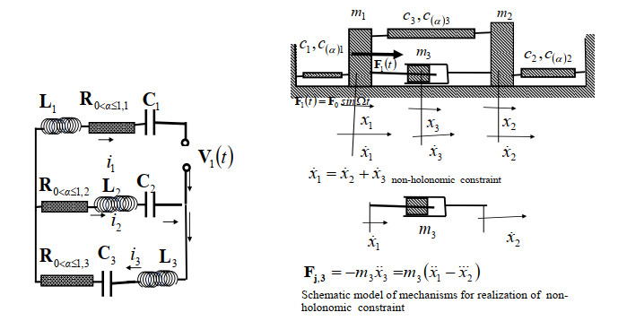
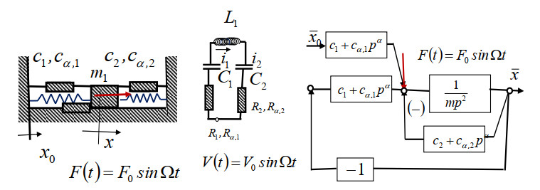
Following the ideas about analogies, mathematical, qualitative, and structural, introduced by Mihailo Petrović in Elements of Mathematical Phenomenology (Serbian Royal Academy, Belgrade, 1911), in this paper we present our research results focused on analogies of fractional-type oscillation models between mechanical and electrical oscillators, with a finite number of degrees of freedom of oscillation. In addition to reviewing basic results, we investigate new constitutive relations and generalizations of the energy dissipation function, mechanical dissipative element of fractional type, and electrical resistor of dissipative fractional type. Those constitutive relations are expressed by means of the fractional order differential operator. By applying the Laplace transformation and the power series expansions, we determine and graphically present the approximate analytical solutions for eigen oscillations of the fractional type, as well as for forced oscillations, using a convolution integral. Tables with elements of mathematical phenomenology and analogies of oscillatory mechanical and electrical systems of fractional type are shown, as well as the principal fractional-type eigen-modes for a class of discrete mechanical or electrical oscillators, when these fractional-type modes are independent and there is no interaction between them. A number of theorems on the properties of independent modes of fractional type and the energy analysis of the discrete systems are also given.

References

[1]	M. Petrović, Elements of Mathematical Phenomenology, Serbian Royal Academy, Belgrade, 1911.
[2]	M. Pétrovitch, Mécanismes communs aux phénomènes disparates, Nouvelle collection scientifique, Félix Alcan, Paris, 1921.
[3]	M. Petrović, Phenomenological Mapping, Serbian Royal Academy, Belgrade, 1933.
[4]	K. R. (Stevanović) Hedrih, The analogy between the stress state model, the strain state model and the mass inertia moment state model, Facta Univ. Ser. Mech. Automat. Control Robot., 1 (1991), 105–120.
[5]	K. R. (Stevanović) Hedrih, Mathematical analogy and phenomenological mapping: Vibrations of multi plate and multi beam homogeneous systems, In: L. Bereteu, T. Cioara, M. Toth-Tascau, C. Vigaru, Editors. Scientific Buletletin of the "Politehnica" University of Timisoara, Romania, Transaction on Mechanics, Editura Politehnica, 50 (2005), Special Issue, 11–18.
[6]	K. R. (Stevanović) Hedrih, Elements of mathematical phenomenology: Ⅰ. Mathematical and qualitative analogies, Trudy MAI, 84 (2015), 1–42.
[7]	K. R. (Stevanović) Hedrih, Elements of mathematical phenomenology: Ⅱ. Phenomenological approximate mappings, Trudy MAI, 84 (2015), 1–29.
[8]	K. R. (Stevanović) Hedrih, J. D. Simonović, Structural analogies on systems of deformable bodies coupled with non-linear layers, Internat. J. Non-Linear Mech., 73 (2015), 18–24. https://doi.org/10.1016/j.ijnonlinmec.2014.11.004 doi: 10.1016/j.ijnonlinmec.2014.11.004
[9]	K. R. (Stevanović) Hedrih, M. Kojić, N. Filipović, Master Class–Serbian Mechanicians, Serbian Society for Mechanics, Belgrade, 2023.
[10]	K. R. (Stevanović) Hedrih, I. Kosenko, P. Krasilnikov, P. D. Spanos, Elements of mathematical phenomenology and phenomenological mapping in non-linear dynamics, Internat. J. Non-Linear Mech., Special issue, 73 (2015), 1–128. https://doi.org/10.1016/j.ijnonlinmec.2015.04.009
[11]	Ž. Mijajlović, S. Pilipović, G. Milovanović, M. Mateljević, M. Albijanić, V. Andrić, et al, Mihailo Petrović Alas: Life, Work, Times–On the Occasion of the 150th Anniversary of his Birth, Serbian Academy of Sciences and Arts, Belgrade, 2019.
[12]	V. Dragović, I. Goryuchkina, About the cover: the Fine-Petrović polygons and the Newton-Puiseux method for algebraic ordinary differential equations, Bull. Amer. Math. Soc., 57 (2020), 293–299.
[13]	F. A. Firestone, A new analogy between mechanical and electrical systems, J. Acoust. Soc. Am., 4 (1933), 249–267. https://doi.org/10.1121/1.1915605 doi: 10.1121/1.1915605
[14]	J. López-Martz, D. García-Vallejo, A. Alcayde, S. Sánchez-Salinas, F. G. Montoya, A comprehensive methodology to obtain electrical analogues of linear mechanical systems, Mech Syst Signal Pr, 200 (2023), 110511. https://doi.org/10.1016/j.ymssp.2023.110511 doi: 10.1016/j.ymssp.2023.110511
[15]	K. R. (Stevanović) Hedrih, Partial fractional order differential equations of transversal vibrations of creep connected double plates systems, In: Workshop Preprints/Proceedings No 2004-1 IFAC FDA 04, ENSEIRB, Bordeaux, France, 2004.
[16]	K. R. (Stevanović) Hedrih, A. N. Hedrih, The Kelvin-Voigt visco-elastic model involving a fractional-order time derivative for modelling torsional oscillations of a complex discrete biodynamical system, Acta Mech., 234 (2023), 1923–1942. https://doi.org/10.1007/s00707-022-03461-7 doi: 10.1007/s00707-022-03461-7
[17]	K. R. (Stevanović) Hedrih, J. A. Tenreiro Machado, Discrete fractional order system vibrations, Internat. J. Non-Linear Mech., 73 (2015), 2–11. http://dx.doi.org/10.1016/j.ijnonlinmec.2014.11.009 doi: 10.1016/j.ijnonlinmec.2014.11.009
[18]	O. A. Goroško, K. R. (Stevanović) Hedrih, Analytical Dynamics (Mechanics) of Discrete Hereditary Systems, University of Niš, 2001.
[19]	A. V. Letnikov, Theory of differentiation with an arbitrary index, Mat. Sb., 3 (1868), 1–66.
[20]	A. V. Letnikov, An explanation of the concepts of the theory of differentiation of arbitrary index, Mat. Sb., 6 (1872), 413–445.
[21]	S. G. Samko, A. A. Kilbas, O. I. Marichev, Fractional Integrals and Derivatives–Theory and Applications, Gordon and Breach Science Publishers, Amsterdam, 1993.
[22]	B. S. Bačlić, T. M. Atanacković, Stability and creep of a fractional derivative order viscoelastic rod, Bull. Cl. Sci. Math. Nat. Sci. Math., 25 (2000), 115–131.
[23]	Yu. N. Rabotnov, Creep Problems in Structural Members, Series in Applied Mathematics and Mechanics, North-Holland, Amsterdam, 1969.
[24]	J. E. Escalante-Martínez, J. F. Gómez-Aguilar, C. Calderón-Ramón, L. J. Morales-Mendoza, I. Cruz-Orduña, J. R. Laguna-Camacho, Experimental evaluation of viscous damping coefficient in the fractional underdamped oscillator, Adv. Mech. Eng., 8 (2016), 1–12. https://doi.org/10.1177/1687814016643068 doi: 10.1177/1687814016643068
[25]	J. F. Gómez-Aguilar, H. Yépez-Martz, C. Calderón-Ramón, I. Cruz-Orduña, R. F. Escobar-Jiménez, V. H. Olivares-Peregrino, Modeling of a mass-spring-damper system by fractional derivatives with and without a singular kernel, Entropy, 17 (2015), 6289–6303. https://doi.org/10.3390/e17096289 doi: 10.3390/e17096289
[26]	J. F. Gómez-Aguilar, Analytic solutions and numerical simulations of mass-spring and damper-spring systems described by fractional differential equations, Rom. J. Phys., 60 (2015), 311–323.
[27]	J. F. Gómez-Aguilar, J. J. Rosales, J. J. Bernal, Mathematical modelling of the mass-spring-damper system – A fractional calculus approach, Acta Universitaria, 22 (2012), 5–11. https://doi.org/10.15174/au.2012.328 doi: 10.15174/au.2012.328
[28]	J. F. Gómez-Aguilar, J. J. Rosales-García, J. J. Bernal-Alvarado, T. Córdova-Fraga, R. Guzmán-Cabrera, Fractional mechanical oscillators, Revista Mexicana de Fca, 58 (2012), 348–352.
[29]	K. B. Oldham, J. Spanier, The Fractional Calculus, Academic Press, New York, 1974.
[30]	B. Ross, A brief history and exposition of the fundamental theory of fractional calculus, In: Fractional Calculus and Its Applications: Proceedings of the International Conference Held at the University of New Haven, June 1974, Springer, Berlin, Heidelberg, 1–36, 2006. https://doi.org/10.1007/BFb0067096
[31]	K. S. Miller, B. Ross, An Introduction to the Fractional Calculus and Fractional Differential Equations, Wiley, New York, 1993.
[32]	L. Debnath, A brief historical introduction to fractional calculus, Internat. J. Math. Ed. Sci. Tech., 35 (2004), 487–501. https://doi.org/10.1080/00207390410001686571 doi: 10.1080/00207390410001686571
[33]	A. A. Kilbas, H. M. Srivastava, J. J. Trujillo, Theory and Applications of Fractional Differential Equations, Elsevier, 2006.
[34]	M. Lazarević, M. Rapaić, T. Šekara, Introduction to Fractional Calculus with Brief Historical Background, In: Advanced Topics on Applications of Fractional Calculus on Control Problems, System Stability and Modeling, 2014, 3–16.
[35]	F. Mainardi, Fractional Calculus and Waves in Linear Viscoelasticity. An Introduction to Mathematical Models, Imperial College Press, London, 2010. https://doi.org/10.1142/9781848163300
[36]	V. Kiryakova, A brief story about the operators of generalized fractional calculus, Fract. Calc. Appl. Anal., 11 (2008), 203–220.
[37]	R. Herrmann, Fractional Calculus–An Introduction For Physicists, World Scientific, Singapore, 2014. https://doi.org/10.1142/8934
[38]	T. Sandev, Ž. Tomovski, Fractional Equations and Models. Theory and applications, Springer Cham, 2019. https://doi.org/10.1007/978-3-030-29614-8
[39]	S. Wolfram, The Mathematica Book, Wolfram Media. Inc., 2003.
[40]	R. Garrappa, M. Popolizio, Evaluation of generalized Mittag-Leffler functions on the real line, Adv. Comput. Math., 39 (2013), 205–225. https://doi.org/10.1007/s10444-012-9274-z doi: 10.1007/s10444-012-9274-z
[41]	R. Gorenflo, J. Loutchko, Y. Luchko, Computation of the Mittag-Leffler function and its derivatives, Fract. Calc. Appl. Anal., 5 (2002), 491–518.
[42]	M. J. Luo, G. V. Milovanović, P. Agarwal, Some results on the extended beta and extended hypergeometric functions, Appl. Math. Comput., 248 (2014), 631–651. https://doi.org/10.1016/j.amc.2014.09.110. doi: 10.1016/j.amc.2014.09.110
[43]	G. V. Milovanović, A. K. Rathie, On a quadratic transformation due to Exton and its generalization, Hacet. J. Math. Stat., 48 (2019), 1706–1711.
[44]	G. V. Milovanović, A. K. Rathie, N. M. Vasović, Summation identities for the Kummer confluent hypergeometric function ${}_1F_1(a, b, ;z)$, Kuwait J. Sci., 50 (2023), 190–193. https://doi.org/10.1016/j.kjs.2023.05.014 doi: 10.1016/j.kjs.2023.05.014
[45]	S. Das, Functional Fractional Calculus, Springer Berlin, Heidelberg, 2011. https://doi.org/10.1007/978-3-642-20545-3
[46]	J. T. Machado, V. Kiryakova, F. Mainardi, Recent history of fractional calculus, Commun. Nonlinear Sci. Numer. Simulat., 16 (2011), 1140–1153. https://doi.org/10.1016/j.cnsns.2010.05.027 doi: 10.1016/j.cnsns.2010.05.027
[47]	S. F. Lacroix, Traité du Calcul Différentiel et du Calcul Intégral, Courcier, Paris, 1819.
[48]	T. M. Atanacković, S. Pilipović, B. Stanković, D. Zorica, Fractional Calculus with Applications in Mechanics: vibrations and diffusion processes, John Wiley & Sons, 2014.
[49]	D. Baleanu, K. Diethelm, E. Scalas, J. J. Trujillo, Fractional Calculus: Models and Numerical Methods, World Scientific, Singapore, 2012.
[50]	G. V. Milovanović, Müntz orthogonal polynomials and their numerical evaluation, in Applications and Computation of Orthogonal Polynomials, Birkhäuser, (1999), 179–202.
[51]	G. V. Milovanović, A. S. Cvetković, Gaussian type quadrature rules for Müntz systems, SIAM J. Sci. Comput., 27 (2005), 893–913. https://doi.org/10.1137/040621533 doi: 10.1137/040621533
[52]	P. Mokhtary, F. Ghoreishi, H. M. Srivastava, The Müntz-Legendre tau method for fractional differential equations, Appl. Math. Modelling, 40 (2016), 671–684. https://doi.org/10.1016/j.apm.2015.06.014 doi: 10.1016/j.apm.2015.06.014
[53]	V. Kiryakova, Generalized Fractional Calculus and Applications, Pitman Research Notes in Mathematics Series, 301, Longman Sci. Tech., Harlow, 1994.
[54]	C. Li, F. Zeng, Numerical Methods for Fractional Calculus, CRC Press, 2015. https://doi.org/10.1201/b18503
[55]	G. Mastroianni, G. V. Milovanović, Interpolation Processes–Basic Theory and Applications, Springer Monographs in Mathematics, Springer Berlin, Heidelberg, 2008. https://doi.org/10.1007/978-3-540-68349-0
[56]	G. V. Milovanović, On certain Gauss type quadrature rules, Jñānābha, 44 (2014), 1–8.
[57]	M. R. Rapaić, T. B. Šekara, V. Govedarica, A novel class of fractionally orthogonal quasi-polynomials and new fractional quadrature formulas, Appl. Math. Comput., 245 (2014), 206–219. https://doi.org/10.1016/j.amc.2014.07.084 doi: 10.1016/j.amc.2014.07.084
[58]	G. V. Milovanović, Some orthogonal polynomials on the finite interval and Gaussian quadrature rules for fractional Riemann-Liouville integrals, Math. Methods Appl. Sci., 44 (2021), 493–516. https://doi.org/10.1002/mma.6752 doi: 10.1002/mma.6752
[59]	M. Ciesielski, T. Blaszczyk, The multiple composition of the left and right fractional Riemann-Liouville integrals–analytical and numerical calculations, Filomat, 31 (2017), 6087–6099. https://doi.org/10.2298/FIL1719087C doi: 10.2298/FIL1719087C
[60]	M. Caputo, Linear models of dissipation whose $Q$ is almost frequency independent–Ⅱ, Geophy. J. Int., 13 (1967), 529–539. https://doi.org/10.1111/j.1365-246X.1967.tb02303.x doi: 10.1111/j.1365-246X.1967.tb02303.x
[61]	I. Podlubny, Fractional Differential Equations, Academic Press, New York, 1999.
[62]	H. Jafari, B. Mohammadi, V. Parvaneh, M. Mursaleen, Weak Wardowski contractive multivalued mappings and solvability of generalized $\varphi$-Caputo fractional snap boundary inclusions, Nonlinear Anal. Model. Control, 28 (2023), 1–16. https://doi.org/10.15388/namc.2023.28.32142 doi: 10.15388/namc.2023.28.32142
[63]	S. Esmaeili, G. V. Milovanović, Nonstandard Gauss-Lobatto quadrature approximation to fractional derivatives, Fract. Calc. Appl. Anal., 17 (2014), 1075–1099. https://doi.org/10.2478/s13540-014-0215-z doi: 10.2478/s13540-014-0215-z
[64]	A. S. Cvetković, G. V. Milovanović, The Mathematica package "OrthogonalPolynomials", Facta Univ. Ser. Math. Inform., 9 (2014), 17–36.
[65]	G. V. Milovanović, A. S. Cvetković, Nonstandard Gaussian quadrature formulae based on operator values, Adv. Comput. Math., 32 (2010), 431–486. https://doi.org/10.1007/s10444-009-9114-y doi: 10.1007/s10444-009-9114-y
[66]	K. Diethelm, The Analysis of Fractional Differential Equations, Springer-Verlag, Berlin, 2010. https://doi.org/10.1007/978-3-642-14574-2
[67]	S. Esmaeili, M. Shamsi, Y. Luchko, Numerical solution of fractional differential equations with a collocation method based on Müntz polynomials, Comput. Math. Appl., 62 (2011), 918–929. https://doi.org/10.1016/j.camwa.2011.04.023 doi: 10.1016/j.camwa.2011.04.023
[68]	P. Novati, Numerical approximation to the fractional derivative operator, Numer. Math., 127 (2014), 539–566. https://doi.org/10.1007/s00211-013-0596-7 doi: 10.1007/s00211-013-0596-7
[69]	D. P. Rašković, Theory of Oscillations, Naučna Knjiga, Beograd, 1965.
[70]	D. P. Rašković, Mechanics III–Dynamics, Naučna Knjiga, Beograd, 1972.
[71]	D. P. Rašković, Analytical Mechanics, Faculty of Mechanical Engineering, Kragujevac, 1974.
[72]	K. Stevanović-Hedrih, A. Ivanović-Šašić, J. Simonović, Lj. Kolar-Anić, Ž. Čupić, Oscillators: Phenomenological mappings and analogies, Second part: Structural analogy and chains, Scientific Technical Review, 65 (2015), 37–45. https://doi.org/10.5937/STR1504037S doi: 10.5937/STR1504037S
[73]	S. V. Eliseev, A. V. Eliseev, Theory of Oscillations: Structural Mathematical Modeling in Problems of Dynamics of Technical Objects, Springer cham, 2020. https://doi.org/10.1007/978-3-030-31295-4

Reader Comments

Your name:*

Email:*
© 2024 the Author(s), licensee AIMS Press. This is an open access article distributed under the terms of the Creative Commons Attribution License (http://creativecommons.org/licenses/by/4.0)