Asymptotic behavior of a viscous incompressible fluid flow in a fractal network of branching tubes

Haifa El Jarroudi; Mustapha El Jarroudi; Haifa El Jarroudi; Mustapha El Jarroudi

doi:10.3934/cam.2024030

Communications in Analysis and Mechanics

2024, Volume 16, Issue 3: 655-699. doi: 10.3934/cam.2024030

Previous Article Next Article

Research article

Asymptotic behavior of a viscous incompressible fluid flow in a fractal network of branching tubes

Haifa El Jarroudi ,
Mustapha El Jarroudi ^,

Department of Mathematics, Abdelmalek Essaâdi University FST Tanger, Tangier, Morocco

Received: 10 January 2024 Revised: 07 March 2024 Accepted: 01 August 2024 Published: 13 September 2024
35B40, 28A80, 35J75

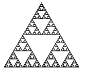
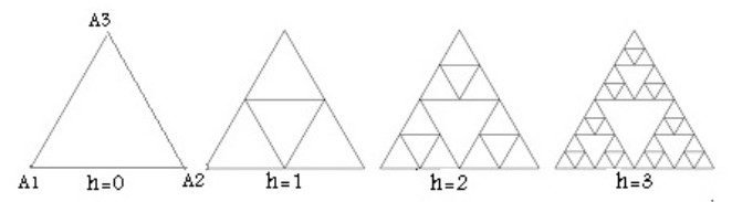
We considered a viscous incompressible fluid flow in a varying bounded domain consisting of branching thin cylindrical tubes whose axes are line segments that form a network of pre-fractal curves constituting an approximation of the Sierpinski gasket. We supposed that the fluid flow is driven by volumic forces and governed by Stokes equations with boundary conditions for the velocity and the pressure on the wall of the tubes and inner continuity conditions for the normal velocity on the interfaces between the junction zones and the rest of the pipes. We constructed local perturbations, related to boundary layers in the junction zones, from solutions of Leray problems in semi-infinite cylinders representing the rescaled junctions. Using $ \Gamma $-convergence methods, we studied the asymptotic behavior of the fluid as the radius of the tubes tends to zero and the sequence of the pre-fractal curves converges in the Hausdorff metric to the Sierpinski gasket. Based on the constructed local perturbations, we derived, according to a critical parameter related to a typical Reynolds number of the flow in the junction zones, three effective flow models in the Sierpinski gasket, consisting of a singular Brinkman flow, a singular Darcy flow, and a flow with constant velocity.
- viscous incompressible fluid flow,
- fractal branching tubes,
- asymptotic behavior,
- critical parameter,
- effective flow models
Citation: Haifa El Jarroudi, Mustapha El Jarroudi. Asymptotic behavior of a viscous incompressible fluid flow in a fractal network of branching tubes[J]. Communications in Analysis and Mechanics, 2024, 16(3): 655-699. doi: 10.3934/cam.2024030

Related Papers:

Abstract

We considered a viscous incompressible fluid flow in a varying bounded domain consisting of branching thin cylindrical tubes whose axes are line segments that form a network of pre-fractal curves constituting an approximation of the Sierpinski gasket. We supposed that the fluid flow is driven by volumic forces and governed by Stokes equations with boundary conditions for the velocity and the pressure on the wall of the tubes and inner continuity conditions for the normal velocity on the interfaces between the junction zones and the rest of the pipes. We constructed local perturbations, related to boundary layers in the junction zones, from solutions of Leray problems in semi-infinite cylinders representing the rescaled junctions. Using $ \Gamma $-convergence methods, we studied the asymptotic behavior of the fluid as the radius of the tubes tends to zero and the sequence of the pre-fractal curves converges in the Hausdorff metric to the Sierpinski gasket. Based on the constructed local perturbations, we derived, according to a critical parameter related to a typical Reynolds number of the flow in the junction zones, three effective flow models in the Sierpinski gasket, consisting of a singular Brinkman flow, a singular Darcy flow, and a flow with constant velocity.

References

[1]	T. J. Pedley, R. C. Schroter, M. F. Sudlow, Flow and pressure drop in systems of repeatedly branching tubes, J. Fluid Mech., 46 (1971), 365–383. https://doi.org/10.1017/S0022112071000594 doi: 10.1017/S0022112071000594
[2]	F. Durst, T. Loy, Investigations of laminar flow in a pipe with sudden contraction of cross sectional area, Comp. Fluids, 13 (1985), 15–36. https://doi.org/10.1016/0045-7930(85)90030-1 doi: 10.1016/0045-7930(85)90030-1
[3]	S. Mayer, On the pressure and flow-rate distributions in tree-like and arterial-venous networks, Bltn. Mathcal. Biology, 58 (1996), 753–785. https://doi.org/10.1007/BF02459481 doi: 10.1007/BF02459481
[4]	M. Blyth, A. Mestel, Steady flow in a dividing pipe, J. Fluid Mech., 401 (1999), 339–364. https://doi.org/10.1017/S0022112099006904 doi: 10.1017/S0022112099006904
[5]	T. J. Pedley, Arterial and venous fluid dynamics, In: G. Pedrizzetti, K. Perktold (eds), Cardiovascular Fluid Mechanics. International Centre for Mechanical Sciences. Springer, Vienna, 446 (2003), 1–72. https://doi.org/10.1007/978-3-7091-2542-7_1
[6]	F. T. Smith, R. Purvis, S. C. R. Dennis, M. A. Jones, N. C. Ovenden, M. Tadjfar, Fluid flow through various branching tubes, J. Eng. Math., 47 (2003), 277–298. https://doi.org/10.1023/B:ENGI.0000007981.46608.73 doi: 10.1023/B:ENGI.0000007981.46608.73
[7]	M. Tadjfar, F. Smith, Direct simulations and modelling of basic three-dimensional bifurcating tube flows, J. Fluid Mech., 519 (2004), 1–32. https://doi.org/10.1017/S0022112004000606 doi: 10.1017/S0022112004000606
[8]	R. I. Bowles, S. C. R. Dennis, R. Purvis, F. T. Smith, Multi-branching flows from one mother tube to many daughters or to a network, Phil. Trans. R. Soc. A., 363 (2005), 1045–1055. https://doi.org/10.1098/rsta.2005.1548 doi: 10.1098/rsta.2005.1548
[9]	G. Panasenko, Partial asymptotic decomposition of domain: Navier-Stokes equation in tube structure, C. R. Acad. Sci., Ser. IIB, Mech. Phys. Astron., 326 (1998), 893–898. https://doi.org/10.1016/S1251-8069(99)80045-3 doi: 10.1016/S1251-8069(99)80045-3
[10]	G. Panasenko, K. Pileckas, Asymptotic analysis of the non-steady Navier-Stokes equations in a tube structure. Ⅰ. The case without boundary-layer-in-time, Nonlinear Anal., 122 (2015), 125–168. https://doi.org/10.1016/j.na.2015.03.008 doi: 10.1016/j.na.2015.03.008
[11]	G. Panasenko, K. Pileckas, Asymptotic analysis of the non-steady Navier-Stokes equations in a tube structure. Ⅱ. General case, Nonlinear Anal., 125 (2015), 582–607. https://doi.org/10.1016/j.na.2015.05.018 doi: 10.1016/j.na.2015.05.018
[12]	E. Marusic-Paloka, Rigorous justification of the Kirchhoff law for junction of thin pipes filled with viscous fluid, Asymptot. Anal., 33 (2003), 51–66.
[13]	M. Lenzinger, Corrections to Kirchhoff's law for the flow of viscous fluid in thin bifurcating channels and pipes, Asymp. Anal., 75 (2011), 1–23. https://doi.org/10.3233/ASY-2011-1048 doi: 10.3233/ASY-2011-1048
[14]	H. Attouch, Variational convergence for functions and operators, Appl. Math. Series, London, Pitman, 1984.
[15]	G. Dal Maso, An introduction to $\Gamma $ -convergence, PNLDEA 8, Birkhäuser, Basel, 1993. https://doi.org/10.1007/978-1-4612-0327-8
[16]	U. Bessi, Another point of view on Kusuoka's measure, Discrete Contin. Dyn. Syst., 41 (2021), 3241–3271. https://doi.org/10.3934/dcds.2020404 doi: 10.3934/dcds.2020404
[17]	M. R. Lancia, M. A. Vivaldi, Asymptotic convergence of transmission energy forms, Adv. Math. Sc. Appl., 13 (2003), 315–341.
[18]	U. Mosco, M. A. Vivaldi, An example of fractal singular homogenization, Georgian Math. J., 14 (2007), 169–194. https://doi.org/10.1515/GMJ.2007.169 doi: 10.1515/GMJ.2007.169
[19]	U. Mosco, M. A. Vivaldi, Fractal reinforcement of elastic membranes, Arch. Rational Mech. Anal., 194 (2009), 49–74. https://doi.org/10.1007/s00205-008-0145-1 doi: 10.1007/s00205-008-0145-1
[20]	R. Capitanelli, M. A. Vivaldi, Insulating layers and Robin problems on Koch mixtures, J. Differential Equations, 251 (2011), 1332–1353.
[21]	U. Mosco, M. A. Vivaldi, Thin fractal fibers, Math. Meth. Appl. Sci., 36 (2013), 2048–2068. https://doi.org/10.1002/mma.1621 doi: 10.1002/mma.1621
[22]	R. Capitanelli, M. R. Lancia, M. A. Vivaldi, Insulating layers of fractal type, Differ. Integ. Equs., 26 (2013), 1055–1076. https://doi.org/10.57262/die/1372858561 doi: 10.57262/die/1372858561
[23]	U. Mosco, M. A. Vivaldi, Layered fractal fibers and potentials, J. Math. Pures Appl., 103 (2015), 1198–1227. https://doi.org/10.1016/j.matpur.2014.10.010 doi: 10.1016/j.matpur.2014.10.010
[24]	R. Capitanelli, M. A. Vivaldi, Reinforcement problems for variational inequalities on fractal sets, Calc. Var., 54 (2015), 2751–2783. https://doi.org/10.1007/s00526-015-0882-6 doi: 10.1007/s00526-015-0882-6
[25]	R. Capitanelli, M. A. Vivaldi, Dynamical quasi-filling fractal layers, Siam J. Math. Anal., 48 (2016), 3931–3961. https://doi.org/10.1137/15M1043893 doi: 10.1137/15M1043893
[26]	S. Creo, Singular p-homogenization for highly conductive fractal layers, Z. Anal. Anwend., 40 (2021), 401–424. https://doi.org/10.4171/ZAA/1690 doi: 10.4171/ZAA/1690
[27]	M. El Jarroudi, Homogenization of a quasilinear elliptic problem in a fractal-reinforced structure, SeMA, 79 (2022), 571–592. https://doi.org/10.1007/s40324-021-00250-5 doi: 10.1007/s40324-021-00250-5
[28]	M. El Jarroudi, Y. Filali, A. Lahrouz, M. Er-Riani, A. Settati, Asymptotic analysis of an elastic material reinforced with thin fractal strips, Netw. Heterog. Media, 17 (2022), 47–72. https://doi.org/10.3934/nhm.2021023 doi: 10.3934/nhm.2021023
[29]	M. El Jarroudi, M. El Merzguioui, M. Er-Riani, A. Lahrouz, J. El Amrani, Dimension reduction analysis of a three-dimensional thin elastic plate reinforced with fractal ribbons, Eur. J. Appl. Math., 34 (2023), 838–869. https://doi.org/10.1017/s0956792523000025 doi: 10.1017/s0956792523000025
[30]	M. J. Lighthill, Physiological fluid dynamics: a survey, J. Fluid Mech. 52 (1972), 475–497. https://doi.org/10.1017/s0022112072001557 doi: 10.1017/s0022112072001557
[31]	J. S. Lee, Y. C. Fung, Flow in nonuniform small blood vessels, Microvascular Res., 3 (1971), 272–287. https://doi.org/10.1016/0026-2862(71)90053-7 doi: 10.1016/0026-2862(71)90053-7
[32]	M. R. Roach, S. Scott, G. G. Ferguson, The hemodynamic importance of the geometry of birfurcations in the circle of Willis (glass model studies), Stroke, 3 (1972), 255–267. https://doi.org/10.1161/01.STR.3.3.255 doi: 10.1161/01.STR.3.3.255
[33]	B. B. Mandelbrot, The Fractal Geometry of Nature, Macmillan, New York, 1983.
[34]	G. B. West, J. H. Brown, B. J. Enquist, A general model for the origin of allometric scaling laws in biology, Science, 276 (1997), 122–126. https://doi.org/10.1126/science.276.5309.122 doi: 10.1126/science.276.5309.122
[35]	Y. Chen, X. Zhang, L. Ren, Y. Geng, G. Bai, Analysis of blood flow characteristics in fractal vascular network based on the time fractional order, Phys. Fluids, 33 (2021), 041902. https://doi.org/10.1063/5.0046622 doi: 10.1063/5.0046622
[36]	M. C. Ruzicka, On dimensionless numbers, Chem. Eng. Res. Desi., 86 (2008), 835–868. https://doi.org/10.1016/j.cherd.2008.03.007 doi: 10.1016/j.cherd.2008.03.007
[37]	E. Marušic-Paloka, A. Mikelic, The derivation of a nonlinear filtration law including the inertia effects via homogenization, Nonl. Anal., 42 (2000), 97–137. https://doi.org/10.1016/S0362-546X(98)00346-0 doi: 10.1016/S0362-546X(98)00346-0
[38]	U. Mosco, Energy functionals on certain fractal structures, J. Conv. Anal., 9 (2000), 581–600.
[39]	H. Schlichting, Boundary Layer Theory, 7th edition, McGraw–Hill, New York, 1979.
[40]	P. M. Gresho, R. L. Sani, On pressure boundary conditions for the incompressible Naviers-Stokes equations, Int. J. Num. Meth. Fluids, 7 (1987), 1111–1145. https://doi.org/10.1002/fld.1650071008 doi: 10.1002/fld.1650071008
[41]	M. Fukushima, Y. Oshima, M. Takeda, Dirichlet Forms and Symmetric Markov Processes, de Gruyter Studies in Mathematics: Vol. 19, Berlin: Eds. Bauer Kazdan, Zehnder, 1994. https://doi.org/10.1515/9783110889741
[42]	J. Kigami, Analysis on Fractals, volume 143 of Cambridge Tracts in Mathematics. Cambridge University Press, Cambridge, 2001.
[43]	M. Fukushima, T. Shima, On a spectral analysis for the Sierpinski gasket, Potential Anal., 1 (1992), 1–35. https://doi.org/10.1007/BF00249784 doi: 10.1007/BF00249784
[44]	U. Mosco, Variational fractals, Ann. Scuola Norm. Sup. Pisa, 25 (1997), 683–712.
[45]	T. Kato, Perturbation Theory for Linear Operators, Springer, Berlin, 1966. https://doi.org/10.1007/978-3-642-53393-8
[46]	J. Kigami, Harmonic metric and Dirichlet form on the Sierpinski gasket, In: K. D. Elworthy, N. Ikeda (eds.), Asymptotic Problems in Probability Theory: Stochastic Models and Diffusions on Fractals, Pitman Research Notes in Math., Longman, London, 283 (1993), 201–218.
[47]	J. Kigami, Measurable Riemannian geometry on the Sierpinski gasket: the Kusuoka measure and the Gaussian heat kernel estimate, Math. Ann., 340 (2008), 781–804. https://doi.org/10.1007/s00208-007-0169-0 doi: 10.1007/s00208-007-0169-0
[48]	S. Kusuoka, Dirichlet forms on fractals and products of random matrices, Publ. Res. Inst. Math. Sci., 25 (1989), 659–680. https://doi.org/10.2977/prims/1195173187 doi: 10.2977/prims/1195173187
[49]	A. Teplyaev, Harmonic coordinates on fractals with finitely ramified cell structure, Canad. J. Math., 60 (2008), 457–480. https://doi.org/10.4153/CJM-2008-022-3 doi: 10.4153/CJM-2008-022-3
[50]	K. Falconer, Techniques in fractal geometry, J. Wiley and sons, Chichester, 1997. https://doi.org/10.2307/2533585
[51]	B. E. Breckner, C. Varga, Elliptic problems on the Sierpinski gasket, In: T. Rassias, L. Tóth (eds), Topics in mathematical analysis and applications, Springer Optimization and Its Applications, 94 (2014), 119–173. https://doi.org/10.1007/978-3-319-06554-0_6
[52]	M. E. Bogovskii, Solutions of some problems of vector analysis associated with the operators div and grad, Trudy Sem. S. L. Sobolev, 80 (1980), 5–40.
[53]	G. P. Galdi, An Introduction to the Mathematical Theory of the Navier–Stokes Equations, I, II, Springer–Verlag, Berlin, 1994.
[54]	E. Marusic-Paloka, The effects of flexion and torsion for the fluid flow through a curved pipe, Appl. Math. Optim., 44 (2001), 245–272. https://doi.org/10.1007/s00245-001-0021-y doi: 10.1007/s00245-001-0021-y

Reader Comments

Your name:*

Email:*
© 2024 the Author(s), licensee AIMS Press. This is an open access article distributed under the terms of the Creative Commons Attribution License (http://creativecommons.org/licenses/by/4.0)