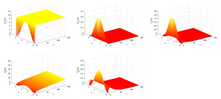
Figure 1.
Evolution of numerical solutions for model (2.11) for R0<1.
Performing their functions as transporters of oxygen and carbon dioxide in the body, human erythrocytes constantly circulate and are exposed to the constant influence of various substances, including nutrients, drugs, medical devices covered with coatings, etc. Therefore, we aim to investigate the biophysical behavior of erythrocytes obtained from healthy volunteers to observe their morphological type changes, alterations in the zeta potential, the electrical conductivity of the erythrocytes in suspensions, and hemolysis in percentages during cells senescence, both in presence and in absence of natural polyelectrolytes pectin (PE) and chitosan (Chi) in form of multilayer films (PEM-films). Being constructed using the layer–by–layer technique, films are an object of interest of many researchers because of their high potential to be incorporated in biomedicine. By applying optical profilometry, electrophoretic light scattering, and spectrophotometry, we tested the polyelectrolytes for any potential harm on the erythrocytes. Based on our results and the one-way analysis of variance (ANOVA) statistical analysis, we reached the conclusion that the above-mentioned polyelectrolytes were harmlessness; therefore, PE and Chi are suitable substances to implement in the clinical practice in the form of drug delivery carriers and medical devices coatings, thereby directly contacting with the human blood.
Citation: Nikolay Kalaydzhiev, Elena Zlatareva, Dessislava Bogdanova, Svetozar Stoichev, Avgustina Danailova. Changes in biophysical properties and behavior of aging human erythrocytes treated with natural polyelectrolytes[J]. AIMS Biophysics, 2025, 12(1): 14-28. doi: 10.3934/biophy.2025002
| [1] | Abhishek Mallick, Atanu Mondal, Somnath Bhattacharjee, Arijit Roy . Application of nature inspired optimization algorithms in bioimpedance spectroscopy: simulation and experiment. AIMS Biophysics, 2023, 10(2): 132-172. doi: 10.3934/biophy.2023010 |
| [2] | Arijit Roy, Abhishek Mallick, Surajit Das, Abhijit Aich . An experimental method of bioimpedance measurement and analysis for discriminating tissues of fruit or vegetable. AIMS Biophysics, 2020, 7(1): 41-53. doi: 10.3934/biophy.2020004 |
| [3] | Svetlana Kashina, Andrea Monserrat del Rayo Cervantes-Guerrero, Francisco Miguel Vargas-Luna, Gonzalo Paez, Jose Marco Balleza-Ordaz . Tissue-specific bioimpedance changes induced by graphene oxide ex vivo: a step toward contrast media development. AIMS Biophysics, 2025, 12(1): 54-68. doi: 10.3934/biophy.2025005 |
| [4] | Tomasz Rok, Artur Kacprzyk, Eugeniusz Rokita, Dorota Kantor, Grzegorz Tatoń . Quantitative assessment of thermal effects on the auricle region caused by mobile phones operating in different modes. AIMS Biophysics, 2024, 11(4): 427-444. doi: 10.3934/biophy.2024023 |
| [5] | Takayuki Yoshida, Hiroyuki Kojima . Subcutaneous sustained-release drug delivery system for antibodies and proteins. AIMS Biophysics, 2025, 12(1): 69-100. doi: 10.3934/biophy.2025006 |
| [6] | Riyaz A. Mir, Jeff Lovelace, Nicholas P. Schafer, Peter D. Simone, Admir Kellezi, Carol Kolar, Gaelle Spagnol, Paul L. Sorgen, Hamid Band, Vimla Band, Gloria E. O. Borgstahl . Biophysical characterization and modeling of human Ecdysoneless (ECD) protein supports a scaffolding function. AIMS Biophysics, 2016, 3(1): 195-210. doi: 10.3934/biophy.2016.1.195 |
| [7] | Neelabh Datta . A review of molecular biology detection methods for human adenovirus. AIMS Biophysics, 2023, 10(1): 95-120. doi: 10.3934/biophy.2023008 |
| [8] | Min Zhang, Shijun Lin, Wendi Xiao, Danhua Chen, Dongxia Yang, Youming Zhang . Applications of single-cell sequencing for human lung cancer: the progress and the future perspective. AIMS Biophysics, 2017, 4(2): 210-221. doi: 10.3934/biophy.2017.2.210 |
| [9] | Mohamed A. Elblbesy . The refractive index of human blood measured at the visible spectral region by single-fiber reflectance spectroscopy. AIMS Biophysics, 2021, 8(1): 57-65. doi: 10.3934/biophy.2021004 |
| [10] | Shivakumar Keerthikumar . A catalogue of human secreted proteins and its implications. AIMS Biophysics, 2016, 3(4): 563-570. doi: 10.3934/biophy.2016.4.563 |
Performing their functions as transporters of oxygen and carbon dioxide in the body, human erythrocytes constantly circulate and are exposed to the constant influence of various substances, including nutrients, drugs, medical devices covered with coatings, etc. Therefore, we aim to investigate the biophysical behavior of erythrocytes obtained from healthy volunteers to observe their morphological type changes, alterations in the zeta potential, the electrical conductivity of the erythrocytes in suspensions, and hemolysis in percentages during cells senescence, both in presence and in absence of natural polyelectrolytes pectin (PE) and chitosan (Chi) in form of multilayer films (PEM-films). Being constructed using the layer–by–layer technique, films are an object of interest of many researchers because of their high potential to be incorporated in biomedicine. By applying optical profilometry, electrophoretic light scattering, and spectrophotometry, we tested the polyelectrolytes for any potential harm on the erythrocytes. Based on our results and the one-way analysis of variance (ANOVA) statistical analysis, we reached the conclusion that the above-mentioned polyelectrolytes were harmlessness; therefore, PE and Chi are suitable substances to implement in the clinical practice in the form of drug delivery carriers and medical devices coatings, thereby directly contacting with the human blood.
Malaria remains a major global health challenge, primarily affecting tropical and subtropical regions. The disease is caused by Plasmodium parasites, transmitted through bites of infected Anopheles mosquitoes. Symptoms include fever, chills, and flu-like illness, and without treatment, malaria can lead to severe complications and death [1]. According to the World Health Organization (WHO), in 2023 there were an estimated 263 million malaria cases and 597,000 malaria deaths worldwide. The African region carries a disproportionately high share of the global malaria burden, accounting for 94% of malaria cases and 95% of malaria deaths [2]. Despite ongoing efforts to control malaria, it continues to be a major global health issue that is especially prevalent in the sub-Saharan African region [3].
Mathematical models are essential for depicting the dynamics of disease transmission and developing effective control strategies [4,5,6]. Early models often assumed a homogeneous environment, ignoring spatial variations such as population density, mosquito distribution, or local ecological conditions. However, newer studies have focused on the importance of spatial heterogeneity in malaria transmission and the need for reaction-diffusion models that incorporate these variations [7]. Spatial heterogeneity significantly impacts malaria transmission, especially in regions with diverse ecological factors. Moreover, delays, such as the incubation periods of malaria in humans and mosquitoes, are crucial components of modern models. These time lags affect the stability and transmission dynamics of malaria. By including these delays in reaction-diffusion malaria models, researchers can better simulate real-world scenarios and assess the effectiveness of control measures over time [8]. For articles on the variable malaria model, please refer to [9,10].
Recent studies have shown promising results with the use of Wolbachia in controlling mosquito-borne diseases, including malaria and dengue. Field trials conducted in various parts of the world have demonstrated that releasing Wolbachia-infected Aedes aegypti mosquitoes can significantly reduce dengue transmission [11]. Similarly, the potential of Wolbachia to control malaria transmission has been explored through laboratory and field studies involving Anopheles mosquitoes, the primary malaria vectors [12]. Moreover, studies in malaria-endemic areas, including regions in Indonesia and Australia, have demonstrated that Wolbachia-infected mosquitoes can successfully integrate into local mosquito populations. This indicates a viable and potentially large-scale strategy for managing malaria [13,14]. Consequently, it is of great importance to investigate the effects of Wolbachia-based methods that disrupt insect reproduction on malaria control efforts.
This paper aims to study the effect of releasing Wolbachia-infected male mosquitoes on malaria control. The paper proceeds with the following structure. The next section details the development of our mathematical model. The well-posedness of the model is studied in Section 3. Section 4 delves into the introduction of the basic reproduction number, denoted as R0. Section 5 focuses on analyzing the threshold dynamics of our model, which are contingent upon the value of R0. Section 6 presents numerical simulations to elucidate the theoretical results, explore the impact of the release ratio of Wolbachia-infected males on transmission and control of malaria, and perform a sensitivity analysis. The paper concludes with a summary in the final section.
The mosquito population has two subclasses: the aquatic population and the winged population. Let L1(x,a1,t) represent wild mosquitoes at time t, position x, and chronological age a1.A(x,t) aquatic mosquitoes at time t and position x. W(x,t) represents female winged mosquitoes at time t and position x. Ω is a bounded region with a smooth boundary ∂Ω. In the aquatic stage, limited habitat space and food resources lead to intense intraspecific competition among the larvae. Consistent with the approach proposed in [15], we utilize the following classic age-structured equations and introduce an additional nonlinear factor to characterize the evolutionary dynamics of mosquito populations under such competition. For t≥0,a1>0
| {(∂∂t+∂∂a1)L1(x,a1,t)=∇⋅(d(x,a1)∇L1(x,a1,t))−g(L1(x,a1,t)),x∈Ω,(d(x,a1)∇L1(x,a1,t))⋅n=0,x∈∂Ω, | (2.1) |
where ∇ indicates the gradient, n is the outward unit normal vector on ∂Ω, d(x,a1) denotes the diffusion coefficient, and g(L1) represents a continuous function of L. The expressions for d(x,a1) and g(L1) are as follows:
| d(x,a1)={0,a1∈(0,τ1],dw(x),a1∈(τ1,+∞).g(L1(x,a1,t))={μa(x)L1(x,a1,t)+c(x)L21(x,a1,t),a1∈(0,τ1],μw(x)L1(x,a1,t),a1∈(τ1,+∞). |
Here, dw signifies the diffusion coefficient for adult mosquitoes. Meanwhile, c indicates the intraspecific competition rate among the larvae, and μa and μw correspond to the natural mortality rates of larvae and adult mosquitoes, respectively. Then A(x,t) and W(x,t) can be determined by integrating the population density over the specified age ranges, as detailed below
| A(x,t)=∫τ10L1(x,a1,t)da1,W(x,t)=∫+∞τ1L1(x,a1,t)da1. | (2.2) |
The female male proportion is assumed to be 1:1. Assuming that Wolbachia-infected male mosquitoes are deployed under a proportional release strategy, that is, the released amount of Wolbachia-infected male mosquitoes is proportional to the current wild male mosquitoes. Here, q(x) represents the ratio of released Wolbachia-infected males to wild males. Let Wc(x,t) be the Wolbachia-infected male mosquitoes. Then we have Wc(x,t)=q(x)W(x,t).
We assume that Wolbachia-infected male mosquitoes have the same mating ability as wild male mosquitoes. Thus, WcW+Wc=q(x)1+q(x) describes the probability of a wild female mosquito mating with Wolbachia-infected male mosquitoes. Then 1−q(x)1+q(x)=11+q(x) is the probability of a wild female mosquito mating with wild male mosquitoes. Denote ρ(x) as the egg-laying rate of each wild females mosquito. We have
| L1(x,0,t)=12ρ(x)11+q(x)W(x,t). |
From (2.1), we can get
| {∂∂tA(x,t)=−μa(x)A(x,t)−c(x)∫τ10L21(x,a1,t)da1+L1(x,0,t)−L1(x,τ1,t),x∈Ω,∂∂tW(x,t)=∇⋅(dm∇W(x,t))−μw(x)W(x,t)+L1(x,τ1,t)−L1(x,+∞,t),x∈Ω. | (2.3) |
It is natural to assume that L1(x,+∞,t)=0. By the characteristic line method, we can obtain the expression of L1(x,τ1,t). If we set w1(x,a1,s)=L1(x,a1,a1+s),a1∈(0,τ1], we have
| {∂∂a1w1(x,a1,s)=(∂∂t+∂∂a1)L1(x,a1,t)|t=a1+s=−μa(x)L1(x,a1,a1+s)−c(x)L21(x,a1,a1+s)=−μa(x)w1(x,a1,s)−c(x)w21(x,a1,s),x∈Ω,w1(x,0,s)=ρ(x)2(1+q(x))W(x,s),x∈Ω. |
We can obtain
| w1(x,a1,s)=w1(x,0,s)e−μa(x)a11+w1(x,0,s)c(x)μa(x)(1−e−μa(x)a1), |
If we let a1=τ1, then s=t−τ1, and we have
| L1(x,τ1,t)=L1(x,0,s)e−μa(x)τ11+L1(x,0,s)c(x)μa(x)(1−e−μa(x)τ1)=ρ(x)2(1+q(x))W(x,t−τ1)e−μa(x)τ11+ρ(x)c(x)2(1+q(x))μa(x)W(x,t−τ1)(1−e−μa(x)τ1). |
Thus, one has
| {∂∂tA(x,t)=−μa(x)A(x,t)−c(x)∫τ10L21(x,a1,t)da1+ρ(x)2(1+q(x))W(x,t)−ρ(x)2(1+q(x))W(x,t−τ1)e−μa(x)τ11+ρ(x)c(x)2(1+q(x))μa(x)W(x,t−τ1)(1−e−μa(x)τ1),∂∂tW(x,t)=∇⋅(dm∇W(x,t))−μw(x)W(x,t)+ρ(x)2(1+q(x))W(x,t−τ1)e−μa(x)τ11+ρ(x)c(x)2(1+q(x))μa(x)W(x,t−τ1)(1−e−μa(x)τ1). | (2.4) |
Let Sw(x,t), Ew(x,t), and Iw(x,t) represent susceptible, exposed, and infectious (female) winged mosquitoes. Thus we have W(x,t)=Sw(x,t)+Ew(x,t)+Iw(x,t). Let Sh(x,t), Eh(x,t), Ih(x,t) and Rh(x,t) represent susceptible, exposed, infectious and recovered humans, respectively. The total density of human population can be expressed by Nh(x,t)=Sh(x,t)+Eh(x,t)+Ih(x,t)+Rh(x,t). Assume that Nh(x,t) satisfies the following equation:
| {∂∂tNh(x,t)=∇⋅(dh(x)∇Nh(x,t))+Λ(x)−μh(x)Nh(x,t),x∈Ω,(dh(x)∇Nh(x,t))⋅n=0,x∈∂Ω, | (2.5) |
where Λ and μh correspond to the influx rate and natural mortality rate of humans, respectively. According to Lemma 1 in [7], system (2.5) has a globally attractive positive steady state, denoted by N∗h(x). In this study, we assume Nh(x,t)≡N∗h(x) for ∀t≥0 and x∈Ω.
Let aw be infection age of winged mosquitoes and Lw(x,aw,t) be the density of infected winged mosquitoes. Then
| {(∂∂t+∂∂aw)Lw(x,aw,t)=∇⋅(dw(x)∇Lw(x,aw,t))−μw(x)Lw(x,aw,t),x∈Ω,(dw(x)∇Lw(x,aw,t))⋅n=0,x∈∂Ω. | (2.6) |
So
| Ew(x,t)=∫τw0Lw(x,aw,t)daw,Iw(x,t)=∫+∞τwLw(x,aw,t)daw. | (2.7) |
From (2.6), we can get
| {∂∂tEw(x,t)=∇⋅(dw(x)∇Ew(x,t))−μw(x)Ew(x,t)+Lw(x,0,t)−Lw(x,τw,t),x∈Ω,∂∂tIw(x,t)=∇⋅(dw(x)∇Iw(x,t))−μw(x)Iw(x,t)+Lw(x,τw,t)−Lw(x,+∞,t),x∈Ω. | (2.8) |
It is natural to assume that Lw(x,+∞,t)=0. By the characteristic line method, we can obtain the expression of Lw(x,τw,t). Set w2(x,aw,s)=Lw(x,aw,aw+s),aw∈(0,τw]. We have
| {∂∂aww2(x,aw,s)=(∂∂t+∂∂aw)Lw(x,aw,t)|t=aw+s=∇⋅(dw(x)∇w2(x,aw,s)))−μw(x)w2(x,aw,s),x∈Ω,w2(x,0,s)=b(x)βhw(x)N∗h(x)Sw(x,s)Ih(x,s),x∈Ω. |
We can obtain
| w2(x,aw,s)=∫ΩΓw(x,y,aw)(b(y)βhw(y)N∗h(y)Sw(y,s)Ih(y,s))dy, |
where Γw is the Green function of the operator ∇⋅(dw(⋅)∇)−μw(⋅) associated with the Neumann boundary condition, b(x) represents bite rate of mosquitoes, βhw(x) represents the transmission probability from infectious humans to adult mosquitoes.
Let aw=τw, then s=t−τw, and
| Lw(x,τw,t)=∫ΩΓw(x,y,τw)(b(y)βhw(y)N∗h(y)Sw(y,t−τw)Ih(y,t−τw))dy. |
We then have
| {∂∂tEw(x,t)=∇⋅(dw(x)∇Ew(x,t))−μw(x)Ew(x,t)+b(x)βhw(x)N∗h(x)Sw(x,t)Ih(x,t)−∫ΩΓw(x,y,τw)(b(y)βhw(y)N∗h(y)Sw(y,t−τw)Ih(y,t−τw))dy,x∈Ω,∂∂tIw(x,t)=∇⋅(dw(x)∇Iw(x,t))−μw(x)Iw(x,t)+∫ΩΓw(x,y,τw)(b(y)βhw(y)N∗h(y)Sw(y,t−τw)Ih(y,t−τw))dy,x∈Ω. | (2.9) |
Let ah be the infection age of humans. Similar to the derivation of ∂Ew(x,t)∂t and ∂Iw(x,t)∂t, we can obtain the following expressions of ∂Eh(x,t)∂t and ∂Ih(x,t)∂t:
| {∂∂tEh(x,t)=∇⋅(dh(x)∇Eh(x,t))−μh(x)Eh(x,t)+b(x)βwh(x)N∗h(x)Sh(x,t)Iw(x,t)−∫ΩΓh(x,y,τh)(b(y)βwh(y)N∗h(y)Sh(y,t−τw)Iw(y,t−τw))dy,x∈Ω,∂∂tIh(x,t)=∇⋅(dh(x)∇Ih(x,t))−(μh(x)+rh(x))Iw(x,t)+∫ΩΓh(x,y,τh)(b(y)βwh(y)N∗h(y)Sh(y,t−τh)I(y,t−τh))dy,x∈Ω, | (2.10) |
where Γh is the Green function of the operator ∇⋅(dh(⋅)∇)−μh(⋅) associated with the Neumann boundary condition, dh represents the diffusion coefficient for humans, βwh represents the transmission probability from infectious mosquitoes to humans, and rh and μh represent recovery rate and death rate of infectious humans, respectively.
In a word, we can obtain the following nonlocal delays reaction-diffusion system:
| ∂∂tA(x,t)=−μa(x)A(x,t)−c(x)∫τ10L21(x,a1,t)da+ρ(x)2(1+q(x))W(x,t)−ρ(x)2(1+q(x))W(x,t−τ1)e−μa(x)τ11+ρ(x)c(x)2(1+q(x))μa(x)W(x,t−τ1)(1−e−μa(x)τ1),∂∂tSw(x,t)=∇⋅(dw(x)∇Sw(x,t))+ρ(x)2(1+q(x))W(x,t−τ1)e−μa(x)τ11+ρ(x)c(x)2(1+q(x))μa(x)W(x,t−τ1)(1−e−μa(x)τ1)−μw(x)Sw(x,t)−b(x)βhw(x)N∗h(x)Sw(x,t)Ih(x,t),∂∂tEw(x,t)=∇⋅(dw(x)∇Ew(x,t))−μw(x)Ew(x,t)+b(x)βhw(x)N∗h(x)Sw(x,t)Ih(x,t)−∫ΩΓw(x,y,τw)(b(y)βhw(y)N∗h(y)Sw(y,t−τw)Ih(y,t−τw))dy,∂∂tIw(x,t)=∇⋅(dw(x)∇Iw(x,t))−μw(x)Iw(x,t)+∫ΩΓw(x,y,τw)(b(y)βhw(y)N∗h(y)Sw(y,t−τw)Ih(y,t−τw))dy,∂∂tSh(x,t)=∇⋅(dh(x)∇Sh(x,t))+Λ(x)−μh(x)Sh(x,t)−b(x)βwh(x)N∗h(x)Sh(x,t)Iw(x,t),∂∂tEh(x,t)=∇⋅(dh(x)∇Eh(x,t))−μh(x)Eh(x,t)+b(x)βwh(x)N∗h(x)Sh(x,t)Iw(x,t)−∫ΩΓh(x,y,τh)(b(y)βwh(y)N∗h(y)Sh(y,t−τw)Iw(y,t−τw))dy, |
| ∂∂tIh(x,t)=∇⋅(dh(x)∇Ih(x,t))−(μh(x)+rh(x))Ih(x,t)+∫ΩΓh(x,y,τh)(b(y)βwh(y)N∗h(y)Sh(y,t−τh)Iw(y,t−τh))dy,∂∂tRh(x,t)=∇⋅(dh(x)∇Rh(x,t))+rh(x)Rh(x,t)−μh(x)Rh(x,t),(dw(x)∇Sw(x,t))⋅n=(dw(x)∇Ew(x,t))⋅n=(dw(x)∇Iw(x,t))⋅n=0,x∈∂Ω,(dh(x)∇Sh(x,t))⋅n=(dh(x)∇Eh(x,t))⋅n=(dh(x)∇Ih(x,t))⋅n=(dh(x)∇Rh(x,t))⋅n=0,x∈∂Ω. |
We know that A(x,t),Eh(x,t), and Rh(x,t) are decoupled from the other equations. Then it can be applied to the following system:
| {∂∂tSw(x,t)=∇⋅(dw(x)∇Sw(x,t))−μw(x)Sw(x,t)+ρ(x)p(x)e−μa(x)τ1W(x,t−τ1)1+ρ(x)p(x)ι(x)(1−e−μa(x)τ1)W(x,t−τ1)−βw(x)Sw(x,t)Ih(x,t),∂∂tEw(x,t)=∇⋅(dw(x)∇Ew(x,t))−μw(x)Ew(x,t)+βw(x)Sw(x,t)Ih(x,t)−∫ΩΓw(x,y,τw)(βw(y)Sw(y,t−τw)Ih(y,t−τw))dy,∂∂tIw(x,t)=∇⋅(dw(x)∇Iw(x,t))−μw(x)Iw(x,t)+∫ΩΓw(x,y,τw)βw(y)Sw(y,t−τw)Ih(y,t−τw)dy,∂∂tSh(x,t)=∇⋅(dh(x)∇Sh(x,t))+Λ(x)−μh(x)Sh(x,t)−βh(x)Sh(x,t)Iw(x,t),∂∂tIh(x,t)=∇⋅(dh(x)∇Ih(x,t))−(μh(x)+rh(x))Ih(x,t)+∫ΩΓh(x,y,τh)βh(y)Sh(y,t−τh)Iw(y,t−τh)dy,(dw(x)∇Sw(x,t))⋅n=(dw(x)∇Ew(x,t))⋅n=(dw(x)∇Iw(x,t))⋅n=0,x∈∂Ω,(dh(x)∇Sh(x,t))⋅n=(dh(x)∇Ih(x,t))⋅n=0,x∈∂Ω, | (2.11) |
where p(x)=12(1+q(x)),ι(x)=c(x)μa(x), βw(x)=b(x)βhw(x)N∗h(x),βh(x)=b(x)βwh(x)N∗h(x).
Let X=C(¯Ω,R5) be the Banach space with the supremum norm ‖⋅‖X, and X+=C(¯Ω,R5+). Let τ=max{τ1,τw,τh}. Define C=C([−τ,0],X) as the Banach space with the norm ‖φ‖=maxθ∈[−τ,0]‖φ(θ)‖X for φ∈C, and C+=C([−τ,0],X+). Then (X,X+) and (C,C+) are strongly ordered Banach spaces. For ς>0 and a function z:[−τ,ς)→X, we define zt∈C by zt(θ)=z(t+θ),θ∈[−τ,0]. Denote Tw(t),Ts(t), and Th(t) : C(¯Ω,R)→C(¯Ω,R) are the evolution operators associated with
| ∂v1∂t=∇⋅(dw(x)∇v1)−μw(x)v1,x∈Ω,∂v2∂t=∇⋅(dh(x)∇v2)−μh(x)v2,x∈Ω,∂v3∂t=∇⋅(dh(x)∇v3)−(μh(x)+rh(x))v3,x∈Ω,(dw(x)∇v1)⋅n=(dh(x)∇v2)⋅n=(dh(x)∇v3)⋅n=0,x∈∂Ω. |
Then, for ϑ∈C(¯Ω,R), one has
| Tw(t)ϑ(x)=∫ΩΓw(x,y,τw)βw(y)ϑ(y)dy,Ts(t)ϑ(x)=∫ΩΓs(x,y,τh)βh(y)ϑ(y)dy,Th(t)ϑ(x)=∫ΩΓh(x,y,τh)βh(y)ϑ(y)dy, |
where Γs is the Green function of the operator ∇⋅(dh(⋅)∇)−μh(⋅) associated with the Neumann boundary condition. We can see that Tj(t) is strongly positive and compact, where j=w,s,h. Set T= diag{Tw(t),Tw(t),Tw(t),Ts(t),Th(t)}. Then T:X→X is a semigroup generated by the operator A= diag {A1,A1,A1,A2,A3} defined on D(A)=D(A1)×D(A1)×D(A1)×D(A2)×D(A3), in which
| D(A1)={ˆϑ∈C2(ˉΩ):(dw(x)∇ˆϑ)⋅n=0on∂Ω},A1ˆϑ=∇⋅(dw(x)∇ˆϑ)−μw(x)ˆϑ,ˆϑ∈D(A1), |
| D(A2)={ˆϑ∈C2(ˉΩ):(dh(x)∇ˆϑ)⋅n=0on∂Ω},A2ˆϑ=∇⋅(dh(x)∇ˆϑ)−μh(x)ˆϑ,ˆϑ∈D(A2), |
| D(A3)={ˆϑ∈C2(ˉΩ):(dh(x)∇ˆϑ)⋅n=0on∂Ω},A3ˆϑ=∇⋅(dh(x)∇ˆϑ)−(μh(x)+rh(x))ˆϑ,ˆϑ∈D(A3). |
For φ=(φ1,φ2,φ3,φ4,φ5)∈C+, define F=(F1,F2,F3,F4,F5):C+→X as
| F1φ(x)=ρ(x)p(x)e−μa(x)τ1(φ1(x,−τ1)+φ2(x,−τ1)+φ3(x,−τ1))1+ρ(x)p(x)ι(x)(1−e−μa(x)τ1)(φ1(x,−τ1)+φ2(x,−τ1)+φ3(x,−τ1))−βw(x)φ1(x,0)φ5(x,0),F2φ(x)=βw(x)φ1(x,0)φ5(x,0)−∫ΩΓw(x,y,τw)(βw(y)φ1(y,−τw)φ5(y,−τw))dy,F3φ(x)=∫ΩΓw(x,y,τw)(βw(y)φ1(y,−τw)φ5(y,−τw))dy,F4φ(x)=Λ(x)−βh(x)φ3(x,0)φ4(x,0),F5φ(x)=∫ΩΓh(x,y,τh)(βh(y)φ4(y,−τh)φ3(y,−τh))dy. |
Then system (2.11) can be rewritten as an abstract functional equation as follows:
| {dudt=Au+F(ut),t>0,u0=φ∈C+. |
where u:=(Sw,Ew,Iw,Sh,Ih).
According to Corollary 8.1.3 in [16] and Corollary 4 in [17], we can get the following lemma.
Lemma 3.1. System (2.11) with an initial value function φ∈C+ has a unique mild solution u(⋅,t,φ) on its maximal interval of existence [0,tφ). Moreover, u(⋅,t,φ)∈C+ for any t∈[0,tφ), and u(⋅,t,φ) is a classical solution of system (2.11) for t>τ.
Lemma 3.2. System (2.11) with an initial value function φ∈C+ has a unique global classical solution u(⋅,t,φ) with u0=φ for t∈[0,∞). Moreover, the solution semiflow Υ(t)=ut(⋅):C+→C+ has a compact global attractor in C+.
Proof. From the first and fourth equations of (2.11), we have
| {∂∂tSw(x,t)≤∇⋅(dm∇Sw(x,t))+e−μa(x)τ1ι(x)(1−e−μa(x)τ1)−μw(x)Sw(x,t),∂∂tSh(x,t)≤∇⋅(dh(x)∇Sh(x,t))+Λ(x)−μh(x)Sh(x,t),(dw(x)∇Sw(x,t))⋅n=(dh(x)∇Sh(x,t))⋅n=0,x∈∂Ω. |
So, for any φ∈C+, Kw,Kh>0 and t0=t0(φ)>0 exist such that Sw(⋅,t,φ)≤Kw and Sh(⋅,t,φ)≤Kh for ∀t≥t0.
Assume M1(t)=∫ΩSw(x,t)dx,M2(t)=∫ΩEw(x,t)dx,M3(t)=∫ΩIw(x,t)dx,M4(t)=∫ΩSh(x,t)dx,M5(t)=∫ΩIh(x,t)dx. Integrating Sw(x,t) in system (2.11), we can obtain
| dM1(t)dt≤∫Ω(e−μa(x)τ1ι(x)(1−e−μa(x)τ1)−μw(x)Sw(x,t))dx−∫Ωβw(x)Sw(x,t)Ih(x,t)dx≤K1∣Ω∣−μw_M1(t)−∫Ωβw(x)Sw(x,t)Ih(x,t)dx,t≥0, |
where K1=e−μa_τ1ι_(1−e−μa_τ1). Thus
| ∫Ωβw(x)Sw(x,t)Ih(x,t)dx≤K1∣Ω∣−μw_M1(t)−dM1(t)dt,t≥0. |
Integrating Ew(x,t) in system (2.11), we can obtain
| dM2(t)dt≤∫Ωβw(x)Sw(x,t)Ih(x,t)dx−μw_M2(t)≤K1∣Ω∣−μw_M1(t)−dM1(t)dt−μw_M2(t),t≥0. |
We can then get
| ddt(M1(t)+M2(t))≤K1∣Ω∣−μw_(M1(t)+M2(t)),t≥0. |
It implies that
| M2(t)≤K1∣Ω∣μw_+e−μw_t(M1(0)+M2(0)),t≥0. |
So, M2(t) is uniformly bounded.
Since Γw(⋅,⋅,⋅) is bounded, by integrating Iw(x,t) in system (2.11), we can obtain
| dM3(t)dt≤−μw_M3(t)+K2∫Ω(βw(y)Sw(y,t−τw)Ih(y,t−τw))dy≤−μw_M3(t)+K2(K1∣Ω∣−μa_M1(t−τw)−dM1(t−τw)dt),t≥τ, |
for some positive constant K2. One then has
| ddt(M3(t)+K2M1(t−τw))≤K1K2∣Ω∣−μ1_(M3(t)+K2M1(t−τw)),t≥τ, |
where μ1_=min{μw_,μa_}. It imply that there are a φ−dependent positive constant K3 and a φ−independent positive constant K4 such that
| M3(t)≤M3(t)+K2M1(t−τw)≤K3(φ)e−μ1_t+K4,t≥τ. |
So, M3(t) is uniformly bounded.
Similarly, we can obtain
| dM4(t)dt≤¯Λ∣Ω∣−μh_M4(t)−∫Ωβh(x)Sh(x,t)Iw(x,t)dx,t≥0. |
Thus
| ∫Ωβh(x)Sh(x,t)Iw(x,t)dx≤¯Λ∣Ω∣−μh_M4(t)−dM4(t)dt,t≥0. |
Since Γh(⋅,⋅,⋅) is bounded, by integrating Ih(x,t) in system (2.11), we can obtain
| dM5(t)dt≤−(μh_+rh_)M5(t)+K5(¯Λ∣Ω∣−μh_M4(t−τh)−dM4(t−τh)dt),t≥τ, |
for some positive constant K5. One then has
| ddt(M5(t)+K5M4(t−τw))≤K5¯Λ∣Ω∣−μh_(M5(t)+K5M4(t−τw)),t≥τ. |
It imply that there are a φ−dependent positive constant K6 and a φ−independent positive constant K7
| M5(t)≤K6(φ)e−μh_t+K7,t≥τ. |
So, M5(t) is uniformly bounded. By the comparison theorem for delayed parabolic equations [16], we find that there exist φ−independent positive number K8,K9,K10 and t1=t1(φ)>t0(φ)+τ such that Ew(⋅,t,φ)≤K8, Iw(⋅,t,φ)≤K9 and Ih(⋅,t,φ)≤K10 for any t≥t1. So, the solution of system (2.11) is global and the solution semiflow Υ(t)=ut(⋅):C+→C+ is point dissipative by Theorem 2.1.8 in [16]. Based on Theorem 3.4.8 in [18], Υ(t) has a compact global attractor in C+ for t≥0.
Set Ew=Iw=Ih=0 in system (2.11). Then, Sw(x,t) satisfies the following system:
| {∂∂tSw(x,t)=∇⋅(dw(x)∇Sw(x,t))−μw(x)Sw(x,t)+ρ(x)p(x)e−μa(x)τ1Sw(x,t−τ1)1+ρ(x)p(x)ι(x)(1−e−μa(x)τ1)Sw(x,t−τ1),(dw(x)∇Sw(x,t))⋅n=0,x∈∂Ω. | (4.1) |
By Theorem 11 in [19] and Lemma 2.1 in [20], system (4.1) admits a globally attractive positive steady state W∗(x). It is easy to know that system (2.11) has an infection-free steady state E0(x)=(W∗(x),0,0,N∗h(x),0). Linearizing system (2.11) at E0(x), we can get
| {∂∂tIw(x,t)=∇⋅(dw(x)∇Iw(x,t))−μw(x)Iw(x,t)+∫ΩΓw(x,y,τw)βw(y)W∗(y)Ih(y,t−τw)dy,∂∂tIh(x,t)=∇⋅(dh(x)∇Ih(x,t))−(μh(x)+rh(x))Ih(x,t)+∫ΩΓh(x,y,τh)b(y)βwh(y)Iw(y,t−τh)dy,(dw(x)∇Iw(x,t))⋅n=(dh(x)∇Ih(x,t))⋅n=0,x∈∂Ω. | (4.2) |
Consider the following linear nonlocal and cooperative reaction-diffusion system:
| {∂∂tIw(x,t)=∇⋅(dw(x)∇Iw(x,t))−μw(x)Iw(x,t)+∫ΩΓw(x,y,τw)βw(y)W∗(y)Ih(y,t)dy,∂∂tIh(x,t)=∇⋅(dh(x)∇Ih(x,t))−(μh(x)+rh(x))Ih(x,t)+∫ΩΓh(x,y,τh)b(y)βwh(y)Iw(y,t)dy,(dw(x)∇Iw(x,t))⋅n=(dh(x)∇Ih(x,t))⋅n=0,x∈∂Ω. | (4.3) |
Substituting Iw(x,t)=eλtψ1(x) and Ih(x,t)=eλtψ2(x) into (4.2) and (4.3), we have
| {λψ1(x)=∇⋅(dw(x)∇ψ1(x))−μw(x)ψ1(x)+e−λτw∫ΩΓw(x,y,τw)βw(y)W∗(y)ψ1(y)dy,λψ2(x)=∇⋅(dh(x)∇ψ2(x))−(μh(x)+rh(x))ψ2(x)+e−λτh∫ΩΓh(x,y,τh)b(y)βwh(y)ψ2(y)dy,(dw(x)∇ψ1(x))⋅n=(dh(x)∇ψ2(x))⋅n=0,x∈∂Ω, | (4.4) |
and
| {λψ1(x)=∇⋅(dw(x)∇ψ1(x))−μw(x)ψ1(x)+∫ΩΓw(x,y,τw)βw(y)W∗(y)ψ1(y)dy,λψ2(x)=∇⋅(dh(x)∇ψ2(x))−(μh(x)+rh(x))ψ2(x)+∫ΩΓh(x,y,τh)b(y)βwh(y)ψ2(y)dy,(dw(x)∇ψ1(x))⋅n=(dh(x)∇ψ2(x))⋅n=0,x∈∂Ω. | (4.5) |
By similar methods to Theorem 7.6.1 in [21], we can see that (4.5) has a principal eigenvalue λ0(W∗) with strongly positive eigenfunctions. λ0(W∗) varies continuously under small perturbations W∗. Similar to Lemma 2.1 in [22], we can obtain the next lemma.
Lemma 4.1. The eigenvalue problem (4.4) admits principal eigenvalues associated with a strongly positive eigenfunction, denoted ˜λ0(W∗,τ). Moreover, ˜λ0(W∗,τ) and λ0(W∗) have the same sign.
Assume ϕ(x):=(ϕw(x),ϕh(x)). Assume that ϕ(x) is the spatial distribution of the initial infective female winged mosquitos and humans. It is easy to see that the distribution of those infective individuals at time t>0 is described by T(t)ϕ(x):=(Tw(t)ϕw(x),Th(t)ϕh(x)). Then the distribution of new infectious female winged mosquitos can be expressed as
| ∫ΩΓw(x,y,τw)βw(y)W∗(y)Th(t)ϕh(y)dy. |
Therefore, the total distribution of infectious female winged mosquitos during the infective period is
| ∫+∞τw∫ΩΓw(x,y,τw)βw(y)W∗(y)Th(t−τw)ϕh(y)dydt=∫+∞0∫ΩΓw(x,y,τw)βw(y)W∗(y)Th(t)ϕh(y)dydt. |
Similarly, the total distribution of infectious humans during the infective period is
| ∫+∞τh∫ΩΓh(x,y,τh)b(y)βwh(y)Tw(t−τh)ϕw(y)dydt=∫+∞0∫ΩΓh(x,y,τh)b(y)βwh(y)Tw(t)ϕw(y)dydt. |
Define the operator F on C(¯Ω,R)×C(¯Ω,R) as
| F(ϕ)(x)=(F1(ϕ)(x),F2(ϕ)(x)),ϕ:=(ϕ1,ϕ2)∈C(¯Ω,R)×C(¯Ω,R),x∈¯Ω, |
where
| F1(ϕ)(x)=∫ΩΓw(x,y,τw)βw(y)W∗(y)ϕ1(y)dy |
and
| F2(ϕ)(x)=∫ΩΓh(x,y,τh)b(y)βwh(y)ϕ2(y)dy. |
Then, we can define the next reproduction operator as
| L=∫+∞0F(T(t)ϕ)dt=F(∫+∞0T(t)ϕdt). |
So, Based on the result in [23], the basic reproduction number R0 can be defined by
| R0:=r(L). | (4.6) |
Additionally, we can get the following lemma.
Lemma 4.2. R0−1 has the same sign as λ0(W∗).
Theorem 5.1. If R0<1, then the infection-free steady state E0(x) of system (2.11) is globally attractive in C+.
Proof. When R0<1, according to Lemmas 4.1 and 4.2, we have ˜λ0(W∗,τ)<0, Since limζ→0˜λ0(W∗+ζ,τ)=˜λ0(W∗,τ), a small enough ζ0>0 exists such that ˜λ0(W∗+ζ0,τ)<0.
Recall that W∗(⋅) is globally attractive for system (4.1), we have lim supt→∞Sw(⋅,t)≤W∗(⋅). So, for some positive constant t0, we have Sw(⋅,t)≤W∗(⋅)+ζ0 for t≥t0. Then, for all t≥t0, we can get
| {∂∂tIw(x,t)≤∇⋅(dw(x)∇Iw(x,t))−μw(x)Iw(x,t)+∫ΩΓw(x,y,τw)βw(y)(W∗(y)+ζ0)+Ih(y,t−τw)dy,∂∂tIh(x,t)≤∇⋅(dh(x)∇Ih(x,t))−(μh(x)+rh(x))Ih(x,t)+∫ΩΓh(x,y,τh)b(y)βwh(y)Iw(y,t−τh)dy,(dw(x)∇Iw(x,t))⋅n=(dh(x)∇Ih(x,t))⋅n=0,x∈∂Ω. | (5.1) |
Set ˜ψ be the strongly positive eigenfunction corresponding to ˜λ0(W∗+ζ0,τ). Then, for t>0, the following linear system
| {∂∂t˜u1(x,t)=∇⋅(dw(x)∇˜u1(x,t))−μw(x)˜u1(x,t)+∫ΩΓw(x,y,τw)βw(y)(W∗(y)+ζ0)+˜u2(y,t−τw)dy,∂∂t˜u2(x,t)=∇⋅(dh(x)∇˜u2(x,t))−(μh(x)+rh(x))˜u2(x,t)+∫ΩΓh(x,y,τh)b(y)βwh(y)˜u1(y,t−τh)dy,(dw(x)∇˜u1(x,t))⋅n=(dh(x)∇˜u2(x,t))⋅n=0,x∈∂Ω, | (5.2) |
admits a solution ˜u(x,t)=e˜λ0(W∗+ζ0,τ)t˜ψ(x). Then, for any given φ∈C+, there is some positive constant ˜m, and one has (Iw(⋅,t,φ),Ih(⋅,t,φ))≤˜m˜u(⋅,t) for all t∈[t0−τ,t0]. According to the comparison principle, we can obtain
| (Iw(x,t,φ),Ih(x,t,φ))≤˜me˜λ0(W∗+ζ0,τ)(t−t0)˜ψ(x),∀t≥t0,x∈¯Ω. |
Therefore, limt→∞(Iw(x,t,φ),Ih(x,t,φ))=(0,0) uniformly for x∈¯Ω. Then Sw(x,t),Ew(x,t),Sh(x,t) in system (2.11) are asymptotic to the following equations
| ∂∂tˆu1(x,t)=∇⋅(dw(x)∇ˆu1(x,t))−μw(x)ˆu1(x,t)+ρ(x)p(x)e−μa(x)τ1ˆu1(x,t−τ1)1+ρ(x)p(x)ι(x)(1−e−μa(x)τ1)ˆu1(x,t−τ1),∂∂tˆu2(x,t)=∇⋅(dw(x)∇ˆu2(x,t))−μw(x)ˆu2(x,t),∂∂tˆu3(x,t)=∇⋅(dh(x)∇ˆu3(x,t))+Λ(x)−μh(x)ˆu3(x,t),(dw(x)∇ˆu1(x,t))⋅n=(dw(x)∇ˆu2(x,t))⋅n=(dw(x)∇ˆu3(x,t))⋅n=0,x∈∂Ω. |
Therefore, limt→∞Ew(x,t,φ)=0, limt→∞Sw(x,t,φ)=W∗(x), limt→∞Sh(x,t,φ)=N∗h(x) uniformly for x∈¯Ω. This completes the proof.
Lemma 5.1. For the solution (Sw(x,t,φ),Ew(x,t,φ),Iw(x,t,φ),Sh(x,t,φ),Ih(x,t,φ)) of system (2.11) with an initial value function φ∈C+.
(i) For any t>0, x∈ˉΩ, one has Sw(x,t,φ)>0 and Sh(x,t,φ)>0. Furthermore, for ∀φ∈C+, there is φ−independent positive constant ζ such that
| lim inft→∞Sw(x,t,φ)≥ζ,lim inft→∞Sh(x,t,φ)≥ζ,uniformlyforx∈ˉΩ. | (5.3) |
(ii) Assume that there exists some t∗≥0 such that Iw(⋅,t∗,φ)≢0 and Ih(⋅,t∗,φ)≢0, then the solution satisfies
| Iw(x,t,φ)>0,Ih(x,t,φ)>0,∀t>t∗,x∈ˉΩ. |
Proof. (i) From Lemma 4.1, for any t>0, x∈ˉΩ and an initial value function φ∈C+, there is an ˘N1>0 such that Sh(x,t,φ)≤˘N1 and Ih(x,t,φ)≤˘N1. Let vw(⋅,t,φ) satisfy
| ∂∂tvw(x,t)=∇⋅(dw(x)∇vw(x,t))−μw(x)vw(x,t)−βw(x)˘N1vw(x,t)+ρ(x)p(x)e−μa(x)τ1vw(x,t−τ1)1+ρ(x)p(x)ι(x)(1−e−μa(x)τ1)vw(x,t−τ1). | (5.4) |
It follows from the comparison principle that
| Sw(⋅,t,φ)≥vw(⋅,t,φ)>0 |
for any t>0 and φ∈C+. By Lemma 2.1 in [20], system (5.4) admits a globally attractive positive steady state v∗w(x). Set ζw=minx∈ˉΩv∗w(x), then we have
| lim inft→∞Sw(x,t,φ)≥ζw,uniformlyforx∈ˉΩ. |
Similarly, from Lemma 4.1, for any t>0, x∈ˉΩ, φ∈C+, there is an ˘N2>0 such that Iw(x,t,φ)≤˘N2.
| ∂∂tSh(x,t)≥∇⋅(dh(x)∇Sh(x,t))+Λ(x)−(μh(x)+βh(x)˘N2)Sh(x,t). | (5.5) |
It follows from the comparison principle that Sh(⋅,t,φ)>0, and there is an ζ<ζw such that lim inft→∞Sh(x,t,φ)≥ζ uniformly for x∈ˉΩ. This implies that (i) holds.
(ii) From system (2.11), we can obtain Iw and Ih, which satisfy
| {∂∂tIw(x,t)≥∇⋅(dw(x)∇Iw(x,t))−μw(x)Iw(x,t),∂∂tIh(x,t)≥∇⋅(dh(x)∇Ih(x,t))−(μh(x)+rh(x))Ih(x,t),(dw(x)∇Iw(x,t))⋅n=(dh(x)∇Ih(x,t))⋅n=0,x∈∂Ω. | (5.6) |
According to the maximum principle, assume some t∗≥0 exists such that Iw(⋅,t∗,φ)≢0 and Ih(⋅,t∗,φ)≢0, and then we have
| Iw(x,t,φ)>0,Ih(x,t,φ)>0,∀t>t∗,x∈ˉΩ. |
This implies that (ii) holds.
Theorem 5.2. The disease is uniformly persistent when R0>1; that is, ϱ>0 exists such that for any initial value function φ∈C+ with φ3(⋅,0)≢0 and φ5(⋅,0)≢0, we have
| lim inft→+∞(Sw(x,t,φ),Ew(x,t,φ),Iw(x,t,φ),Sh(x,t,φ),Ih(x,t,φ))≥(ϱ,ϱ,ϱ,ϱ,ϱ) | (5.7) |
uniformly for x∈ˉΩ.
Proof. Let (Sw(x,t,φ),Ew(x,t,φ),Iw(x,t,φ),Sh(x,t,φ),Ih(x,t,φ)) be the solution of system (2.11) with an initial value function φ∈C+. Set
| S0={φ∈C+:φ3(⋅)≢0andφ5(⋅)≢0},∂S0:=C+∖S0={φ∈C+:φ3(⋅)≡0,orφ5(⋅)≡0}. |
From Lemma 5.1, if φ∈∂S0, then Iw(x,t,φ)>0 and Ih(x,t,φ)>0 for x∈ˉΩ, t>0. So, we have Υ(t)S0⊂S0. Denote S∂={φ∈∂S0:Υ(t)φ∈∂S0,t≥0}.ω(φ) as the omega limit set of the forward orbit γ+(φ):={Υ(t)φ:t≥0}. We divide the proof into the following two claims.
Claim 1. For any φ∈S∂, the omega limit set ω(φ)=E0(x).
For any φ∈S∂, we have Υ(t)φ∈∂S0. Hence, either Iw(⋅,t,φ)≡0 or Ih(⋅,t,φ)≡0 for all t≥0. If Iw(⋅,t,φ)≡0 for all t≥0, then, from the third equation of (2.11), we have Ih(⋅,t,φ)≡0 for all t≥0. Then Ew(⋅,t,φ) satisfies
| {∂∂tEw(x,t)=∇⋅(dw(x)∇Ew(x,t))−μw(x)Ew(x,t),(dw(x)∇Ew(x,t))⋅n=0,x∈∂Ω. |
Thus, limt→∞Ew(x,t,φ)=0, uniformly for x∈ˉΩ. Then, Sw(⋅,t,φ) is asymptotic to the linear system (4.1). So, limt→∞Sw(x,t,φ)=W∗(x) uniformly for x∈ˉΩ. It is easy to know that Sh(⋅,t,φ) satisfies system (2.5). Then, limt→∞Sh(x,t,φ)=N∗h(x) uniformly for x∈ˉΩ. In words,
| limt→∞(Sw(x,t,φ),Ew(x,t,φ),Iw(x,t,φ),Sh(x,t,φ),Ih(x,t,φ))=E0(x),uniformlyforx∈ˉΩ. |
Assume Iw(⋅,t3,φ)≢0 for some t3>0. Then Ih(⋅,t,φ)≡0 for t>t3. From Lemma 5.1, we can obtain Iw(⋅,t,φ)>0 for t>t3. Since Ih(⋅,t,φ)≡0 for t>t3, we have Iw(⋅,t,φ)≡0 for t>t3 from the fifth equation of (2.11). This contradicts our assumption. Therefore, ω(φ)=E0(x) for any φ∈S∂.
Claim 2. E0(x) is a uniform weak repeller for S0, i.e.,
| lim supt→+∞‖Υ(t)φ−E0(⋅)‖≥σ∗,foranyφ∈S0. | (5.8) |
Since R0>1, from Lemma 4.2, λ0(W∗)>0. For any given σ∈(0,min{W_∗,Nh_∗}], set λ0(W∗,σ) be the principal eigenvalue of the nonlocal elliptic eigenvalue problem as follows:
| {λψ1(x)=∇⋅(dw(x)∇ψ1(x))−μw(x)ψ1(x)+∫ΩΓw(x,y,τw)βw(y)(W∗(y)−σ)ψ1(y)dy,λψ2(x)=∇⋅(dh(x)∇ψ2(x))−(μh(x)+rh(x))ψ2(x)+∫ΩΓh(x,y,τh)βh(y)(N∗h(y)−σ)ψ2(y)dy,(dw(x)∇ψ1(x))⋅n=(dh(x)∇ψ2(x))⋅n=0,x∈∂Ω. | (5.9) |
We can then obtain limσ→0+λ0(W∗,σ)=λ0(W∗). So, we can find some sufficiently small constant σ∗∈(0,min{W_∗,Nh_∗}] such that λ0(W∗,σ∗)>0.
If (5.8) is not true, then φ∗∈S0 exists such that lim supt→+∞‖Υ(t)φ−E0(⋅)‖<σ∗. Then some t4>0 exists such that ‖Υ(t)φ−E0(⋅)‖<σ∗ for any t≥t4. So, Sw(⋅,t,φ∗)>W∗(x)−σ∗, Sh(⋅,t,φ∗)>N∗h(x)−σ∗, 0<Ew(⋅,t,φ∗)<σ∗, 0<Iw(⋅,t,φ∗)<σ∗, and 0<Ih(⋅,t,φ∗)<σ∗ for any t≥t4. Then we have
| {∂∂tIw(x,t)≥∇⋅(dw(x)∇Iw(x,t))−μw(x)Iw(x,t)+∫ΩΓw(x,y,τw)βw(y)(W∗(y)−σ∗)Ih(y,t−τw)dy,∂∂tIh(x,t)≥∇⋅(dh(x)∇Ih(x,t))−(μh(x)+rh(x))Ih(x,t)+∫ΩΓh(x,y,τh)βh(y)(N∗h(y)−σ∗)Iw(y,t−τh)dy,(dw(x)∇Iw(x,t))⋅n=(dh(x)∇Ih(x,t))⋅n=0,x∈∂Ω, | (5.10) |
for all t≥t5:=t4+τ.
Set ψ=(ψ1,ψ2) be the positive eigenfunction associated with the principal eigenvalue ˜λ0(W∗,τ,σ∗) of the following eigenvalue problem:
| {λψ1(x)=∇⋅(dw(x)∇ψ1(x))−μw(x)ψ1(x)+e−λτw∫ΩΓw(x,y,τw)βw(y)(W∗(y)−σ∗)ψ1(y)dy,λψ2(x)=∇⋅(dh(x)∇ψ2(x))−(μh(x)+rh(x))ψ2(x)+e−λτh∫ΩΓh(x,y,τh)βh(y)(N∗h(y)−σ∗)ψ2(y)dy,(dw(x)∇ψ1(x))⋅n=(dh(x)∇ψ2(x))⋅n=0,x∈∂Ω. | (5.11) |
From Lemma 4.1, ˜λ0(W∗,τ,σ∗) and λ0(W∗,σ∗) have the same sign. So, ˜λ0(W∗,τ,σ∗)>0. Consider the following the linear system:
| {∂∂tν1(x,t)=∇⋅(dw(x)∇ν1(x,t))−μw(x)ν1(x,t)+∫ΩΓw(x,y,τw)βw(y)(W∗(y)−σ∗)ν2(y,t−τw)dy,∂∂tν2(x,t)=∇⋅(dh(x)∇ν2(x,t))−(μh(x)+rh(x))ν2(x,t)+∫ΩΓh(x,y,τh)βh(y)(N∗h(y)−σ∗)ν1(y,t−τh)dy,(dw(x)∇ν1(x,t))⋅n=(dh(x)∇ν2(x,t))⋅n=0,x∈∂Ω, | (5.12) |
for t≥t5. It is easy to see that system (5.12) has a solution (ν1(x,t),ν2(x,t))=e˜λ0(W∗,τ,σ∗)t((ψ1(x),ψ2(x))). Together (5.10) with the comparison principle, we can see that a sufficiently small positive number L exists such that
| (Iw(x,t),Ih(x,t))≥L(ν1(x,t),ν2(x,t))=Le˜λ0(W∗,τ,σ∗)t((ψ1(x),ψ2(x))),∀t≥t5,x∈ˉΩ. |
Since ˜λ0(W∗,τ,σ∗)>0, we get
| limt→+∞Iw(⋅,t)=∞,limt→+∞Ih(⋅,t)=∞, |
which is a contradiction. Therefore, (5.8) is true.
So, E0(⋅) is an isolated invariant set C+, and WS(E0(⋅))∩S0=∅, in which WS(E0(⋅)) is a stable set of E0(⋅). Define a continuous function f:C+→R+ with the following form:
| f(φ)=min{minx∈ˉΩφ3(x),minx∈ˉΩφ5(x)},∀∈φ∈C+. |
Clearly, f−1(0,+∞)⊂S0. From Lemma 5.1 (ii), we can see that if f(φ)=0 for φ∈S0, or f(φ)>0, then f(Υ(t)(φ))>0 for any t>0. So, f is a generalized distance function for the semiflow Υ(t):C+→C+. By Theorem 3 in [24], we can see that ϱ0>0 exists such that minϑ∈ω(φ)f(ϑ)≥ϱ0 for any φ∈S0. This implies uniform persistence.
In this section, numerical simulations are conducted to validate the analytical outcomes. By [25], we choose H∗(x)=53(km2)−1, the periodicity is set to T=12 months, and Ω=(0,π). The parameter values are as follows: N∗h=50,μh=0.00157, Λ=N∗h×μh, rh=0.08,c=0.000001,ρ=50,μa=9,μw=2,τ1=0.5605,τw=17.25/30.4,τh=15/30.4,dw=0.0125,dh=0.1,
| q(x)=5(1−0.01cos(2x)),βhw(x)=0.6(1−0.01cos(2x)),βwh(x)=0.2(1−0.01cos(2x)). |
We set the initial functions as follows:
| Sw(x,ψ)=5(1−cos(2x)),Ew(x,ψ)=0.2(1−cos(2x)),Iw(x,ψ)=0.3(1−cos(2x)), |
| Sh(x,ψ)=4(1−cos(2x)),Ih(x,ψ)=0.2(1−cos(2x)),ψ∈[−τ,0],x∈[0,π]. |
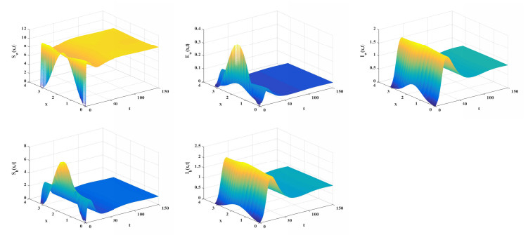
Choose b=5. Numerical simulation determines that R0≈0.2844<1. Based on Theorem 5.1, E0(x) is globally attractive. As shown in Figure 1, the disease will eventually vanish. In other hand, we set b=18. The basic reproduction number can be calculated to be R0≈1.024>1. The dynamic behavior of model (2.11) is illustrated in Figure 2, corroborating the theoretical result of Theorem 5.2. This indicates that an outbreak of the disease is likely to occur.
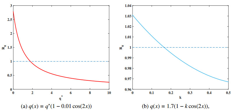
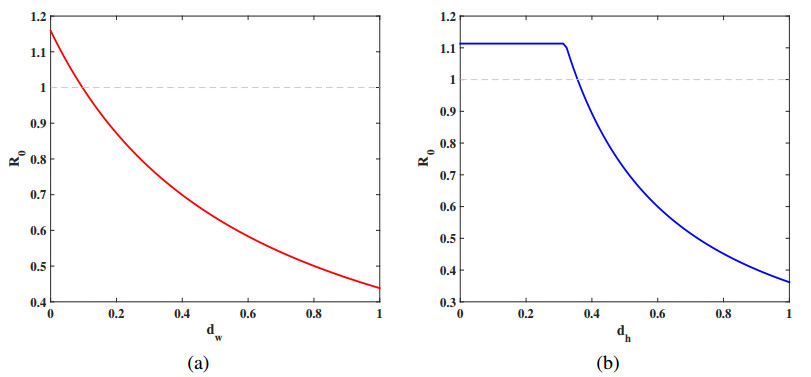
Let q(x)=q∗(1−kcos(2x)), and set b=18,βhw(x)=0.6,βwh(x)=0.2. Firstly, fix k=0.01. We investigate the correlation between q∗ and R0. From Figure 3(a), as q∗ increases, R0 gradually decreases and crosses the threshold of 1. Next, fix q∗=1.7. We analyze the influence of spatial heterogeneity, represented by k, on R0. Figure 3(b) demonstrates that R0 is an increasing function with respect to k. It should be noted that q(x) represents a homogeneous distribution when k=0. Moreover, set q=1.5, we explore the effects of the diffusion rates dw and dh on R0 as shown in Figure 4.
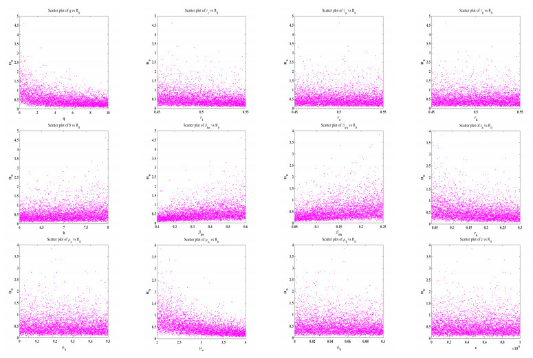
In this part, we explore the situation where the parameters of model (2.11) are constant. By [26], the basic reproduction number R0 can be calculated as
| R0=√b2βhwβwhW∗e−τwμwe−τhμhN∗hμw(μh(x)+rh(x)). |
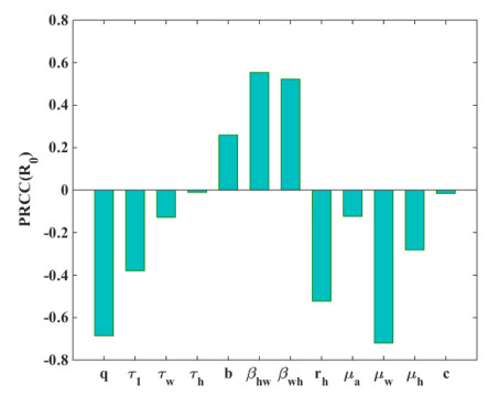
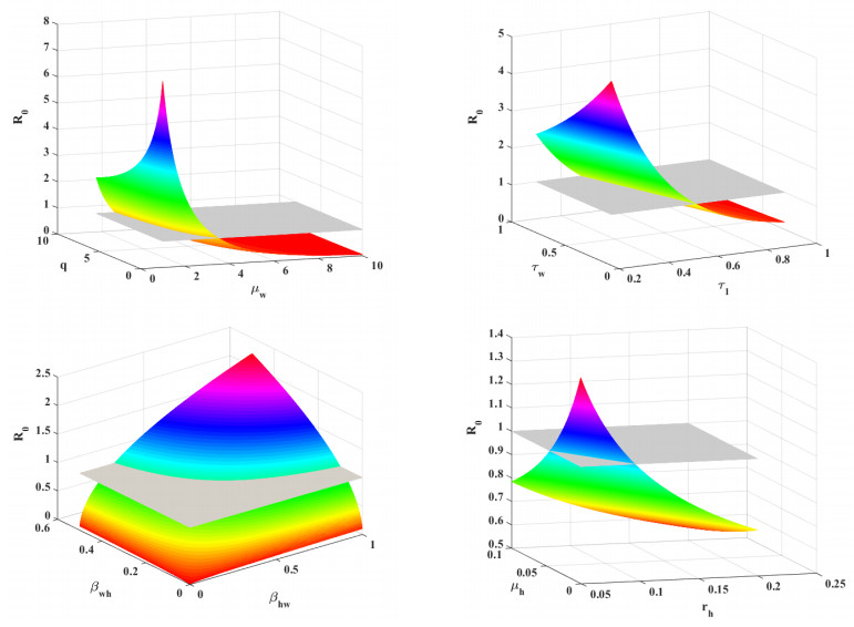
Figure 5 displays scatter plots that illustrate the correlation between the parameters and the basic reproduction number R0. Figure 6 displays a bar chart illustrating the partial rank correlation coefficient (PRCC) values for different parameters in relation to R0. The bars represent the correlation coefficients for each parameter, with some bars above and some below the zero line, indicating positive and negative correlations, respectively. The parameters βhw and βwh show the strong positive correlations, while q, rh and μw show the most negative correlations. The parameter b shows a moderate positive correlation with R0. Additionally, some parameters τ1, τw, and μh show moderate negative correlations. The variations in the remaining parameters have a moderate impact on R0. The contour diagrams in Figure 7 illustrate the joint effect of two parameters on the basic reproduction number R0.
This paper has presented a comprehensive mathematical model for the spatial spread of malaria, incorporating the effects of nonlocal delays and the release of Wolbachia-infected male mosquitoes as a control strategy. The model's dynamics were primarily governed by the basic reproduction number R0, which served as a threshold parameter. Through rigorous theoretical analysis, we established that when R0<1, the infection-free steady state is globally attractive, indicating that malaria can be effectively controlled under this condition. Conversely, when R0>1, the disease persists uniformly, suggesting that malaria will persist in the population. The simulations confirmed the theoretical predictions and provided insights into the impact of the release ratio of Wolbachia-infected males on the transmission and control of malaria. Future research could further explore the integration of Wolbachia release with other vector control methods to optimize malaria elimination efforts.
The authors declare they have not used Artificial Intelligence (AI) tools in the creation of this article.
The work is partially supported by the National Natural Science Foundation of China (No. 12201007), the Natural Science Foundation of Shandong Province (ZR2024QA021), the Natural Science Research Project of Anhui Educational Committee (No. 2022AH050961, 2023AH030021), the Teaching Research Project of Anhui Polytechnic University (No. 2022jyxm67), the Science and Technology Plan Program of Wuhu Municipal (No. 2024kj016).
The authors declare that there are no conflicts of interest.
| [1] |
Kuck L, Peart JN, Simmonds MJ (2020) Active modulation of human erythrocyte mechanics. Am J Physiol Cell Physiol 319: C250-C257. https://doi.org/10.1152/ajpcell.00210.2020 
|
| [2] |
Sakamoto W, Azegami N, Konuma T, et al. (2021) Single-cell native mass spectrometry of human erythrocytes. J Anal Chem 93: 6583-6588. https://doi.org/10.1021/acs.analchem.1c00588
|
| [3] |
Giardina B, Messana I, Scatena R, et al. (1995) The multiple functions of hemoglobin. J Crit Rev Biochem Mol Biol 30: 165-196. https://doi.org/10.3109/10409239509085142
|
| [4] |
Thiagarajan P, Parker CJ, Prchal JT (2021) How do red blood cells die?. J Front Physiol 12: 655393. https://doi.org/10.3389/fphys.2021.655393
|
| [5] |
Dinarelli S, Longo G, Dietler G, et al. (2018) Erythrocyte's aging in microgravity highlights how environmental stimuli shape metabolism and morphology. Sci Rep-UK 8: 5277. https://doi.org/10.1038/s41598-018-22870-0
|
| [6] |
Goodman SR, Hughes KMH, Kakhniashvili DG, et al. (2007) The isolation of reticulocyte-free human red blood cells. J Exp Biol Med (Maywood) 232: 1470. https://doi.org/10.3181/0706-RM-163
|
| [7] |
Pretini V, Koenen MH, Kaestner L, et al. (2019) Red blood cells: chasing interactions. Front Physiol 10: 945. https://doi.org/10.3389/fphys.2019.00945
|
| [8] |
Grebowski J, Kazmierska-Grebowska P, Cichon N, et al. (2022) The effect of fullerenol C60(OH)36 on the antioxidant defense system in erythrocytes. Int J Mol Sci 23: 119. https://doi.org/10.3390/ijms23010119
|
| [9] |
Lawrence C, Meier E (2021) Chapter 17-erythrocyte disorders. Biochemical and Molecular Basis of Pediatric Disease : 529-560. https://doi.org/10.1016/B978-0-12-817962-8.00023-8
|
| [10] |
Maheshwari N, Khan FH, Mahmood R (2019) Pentachlorophenol-induced cytotoxicity in human erythrocytes: enhanced generation of ROS and RNS, lowered antioxidant power, inhibition of glucose metabolism, and morphological changes. Environ Sci Pollut Res 13: 12985-13001. https://doi.org/10.1007/s11356-019-04736-8
|
| [11] |
Piscopo M, Notariale R, Tortora F, et al. (2020) Novel insights into mercury efects on hemoglobin and membrane proteins in human erythrocytes. Molecules 25: 3278. https://doi.org/10.3390/molecules25143278
|
| [12] | Berzuini A, Bianco C, Migliorini AC, et al. (2021) Red blood cell morphology in patients with COVID-19-related anaemia. J Blood Transfus 19: 34-36. https://doi.org/10.2450/2020.0242-20 |
| [13] | Yamaguchi T, Ishimatu T (2020) Effects of cholesterol on membrane stability of human erythrocytes. J Biol Pharm Bull 43: 604-1608. https://doi.org/10.1248/bpb.b20-00435 |
| [14] |
Jan KM, Chien SH (1973) Role of surface electric charge in red blood cell interactions. J Gen Physiol 61: 638-654. https://doi.org/10.1085/jgp.61.5.638
|
| [15] |
Vincy A, Mazumder S, Amrita Banerjee I, et al. (2022) Recent progress in red blood cells-derived particles as novel bioinspired drug delivery systems: challenges and strategies for clinical translation. Front Chem 10: 905256. https://doi.org/10.3389/fchem.2022.905256
|
| [16] |
Tokumasu F, Ostera GR, Amaratunga Ch, et al. (2012) Modifications in erythrocyte membrane zeta potential by plasmodium falciparum Infection. Exp Parasitol 131: 245-251. https://doi.org/10.1016/j.exppara.2012.03.005
|
| [17] | Selim NS (2010) Comparative study on the effect of radiation on whole blood and isolated red blood cells. Romanian J Biophys 20: 127-136. |
| [18] |
Chen XY, Huang YX, Liu W, et al. (2007) Membrane surface charge and morphological and mechanical properties of young and old erythrocytes. J Curr Appl Phys 7: 94-96. https://doi.org/10.1016/j.cap.2006.11.024
|
| [19] |
Kuchinka J, Willems Ch, Telyshev DV, Groth T (2021) Control of blood coagulation by hemocompatible material surfaces—a review. Bioengineering 8: 215. https://doi.org/10.3390/bioengineering8120215
|
| [20] |
Doltchinkova V, Stoylov S, Angelova P (2021) Viper toxins affect membrane characteristics of human erythrocytes. Biophys Chem 270: 106532. https://doi.org/10.1016/j.bpc.2020.106532
|
| [21] |
Qian J, Chen Y, Wang Q, et al. (2021) Preparation and antimicrobial activity of pectin-chitosan embedding nisin microcapsules. Eur Polym J 157: 110676. https://doi.org/10.1016/j.eurpolymj.2021.110676
|
| [22] |
Xie Q, Zheng X, Li L, et al. (2021) Effect of curcumin addition on the properties of biodegradable pectin/chitosan films. Molecules 26: 2152. https://doi.org/10.3390/molecules26082152
|
| [23] |
Jovanović J, Ćirković J, Radojković A, et al. (2021) Chitosan and pectin-based films and coatings with active components for application in antimicrobial food packaging. Prog Org Coat 158: 106349. https://doi.org/10.1016/j.porgcoat.2021.106349
|
| [24] |
Jiang Z, Zhao S, Yang M, et al. (2022) Structurally stable sustained-release microcapsules stabilized by self-assembly of pectin-chitosan-collagen in aqueous two-phase system. J Food Hydrocolloids 125: 107413. https://doi.org/10.1016/j.foodhyd.2021.107413
|
| [25] |
Mallory A, Giannopoulos S, Lee P, et al. (2021) Covered stents for endovascular treatment of aortoiliac occlusive disease: a systematic review and meta-analysis. Vasc Endovasc Surg 55: 560-570. https://doi.org/10.1177/15385744211010381
|
| [26] | Kawagoe Y, Otuka F, Onozuka D, et al. (2022) Early vascular responses to abluminal biodegradable polymer-coated versus circumferential durable polymer-coated newer-generation drug-eluting stents in humans: a pathologic study. EuroIntervention 18: 1284-1294. https://doi.org/10.4244/EIJ-D-22-00650 |
| [27] |
McKenna CG, Vaughan TJ (2022) A computational framework examining the mechanical behaviour of bare and polymer-covered self-expanding laser-cut stents. J Cardiovasc Eng Tech 13: 466-480. https://doi.org/10.1007/s13239-021-00597-w
|
| [28] |
Hu B, Guo Y, Li H, et al. (2021) Recent advances in chitosan-based layer-by-layer biomaterials and their biomedical applications. Carbohyd Polym 271: 118427. https://doi.org/10.1016/j.carbpol.2021.118427
|
| [29] |
Arnon-Ripsb H, Poverenova E (2018) Improving food products' quality and storability by using layer by layer edible coatings. Trends Food Sci Tech 75: 81-92. https://doi.org/10.1016/j.tifs.2018.3.003
|
| [30] |
Grebowski J, Konarska A, Piotrowski P, et al. (2024) Kinetics of metallofullerenol reactions with the products of water radiolysis: implications for radiotherapeutics. ACS Appl Nano Mater 7: 539-549. https://doi.org/10.1021/acsanm.3c04747
|
| [31] |
Silva DCN, Jovino CN, Silva CAL, et al. (2012) Optical tweezers as a new biomedical tool to measure zeta potential of stored red blood cells. Plos One 7: e31778. https://doi.org/10.1371/journal.pone.0031778
|
| [32] |
Raat NJ, Verhoeven AJ, Mik EG (2005) The effect of storage time of human red cells on intestinal microcirculatory oxygenation in a rat isovolemic exchange model. Crit Care Med 33: 39-45. https://doi.org/10.1097/01.ccm.0000150655.75519.02
|
| [33] |
Chen KY, Lin TH, Yang CY, et al. (2018) Mechanics for the adhesion and aggregation of red blood cells on chitosan. J Mechanics 34: 725-732. https://doi.org/10.1017/jmech.2018.27
|
| [34] |
Kou S, Peters L, Mucalo M (2022) Chitosan: a review of molecular structure, bioactivities and interactions with the human body and microorganisms. J Carbohyd Polym 282: 119132. https://doi.org/10.1016/j.carbpol.2022.119132
|
| [35] |
Nadesh R, Narayanan D, Sreerekha PR, et al. (2013) Hematotoxicological analysis of surface-modified and unmodified chitosan nanoparticles. J Biomed Mater Res Part A 101A: 2957-2966. https://doi.org/10.1002/jbm.a.34591
|
| [36] |
Balan V, Verestiuc L (2014) Strategies to improve chitosan hemocompatibility: a review. Eur Polym J 53: 171-188. https://doi.org/10.1016/j.eurpolymj.2014.01.033
|
| [37] |
Zhou X, Zhang X, Zhou J, et al. (2017) An investigation of chitosan and its derivatives on red blood cell agglutination. RSC Adv 7: 12247-12254. https://doi.org/10.1039/C6RA27417
|
| [38] |
Wang W, Xue Ch, Mao X (2020) Chitosan: structural modification, biological activity and application. Int J Biol Macromol 164: 4532-4546. https://doi.org/10.1016/j.ijbiomac.2020.09.042
|
| [39] |
Azmana M, Mahmood S, Hilles AR, et al. (2021) A review on chitosan and chitosan-based bionanocomposites: Promising material for combatting global issues and its applications. Int J Biol Macromol 185: 832-848. https://doi.org/10.1016/j.ijbiomac.2021.07.023
|
| [40] |
Negm NA, Hefni HHH, Abd-Elaal AAA, et al. (2020) Advancement on modification of chitosan biopolymer and its potential applications. Int J Biol Macromol 152: 681-702. https://doi.org/10.1016/j.ijbiomac.2020.02.196
|
| [41] |
Erdogan E, Bajaj R, Lansky A, et al. (2022) Intravascular imaging for guiding in-stent restenosis and stent thrombosis therapy. J Am Heart Assoc 11: e026492. https://doi.org/10.1161/JAHA.122.026492
|
| [42] |
Nagaraja V, Schwarz K, Moss S, et al. (2020) Outcomes of patients who undergo percutaneous coronary intervention with covered stents for coronary perforation: a systematic review and pooled analysis of data. Catheter Cardio Inte 96: 1360-1366. https://doi.org/10.1002/ccd.28646
|
| 1. | Lucian Pîslaru-Dănescu, George-Claudiu Zărnescu, Gabriela Telipan, Victor Stoica, Design and Manufacturing of Equipment for Investigation of Low Frequency Bioimpedance, 2022, 13, 2072-666X, 1858, 10.3390/mi13111858 | |
| 2. | Jiawen Chen, Seyed Mohammad Mir, Maria R. Hudock, Meghan R. Pinezich, Panpan Chen, Matthew Bacchetta, Gordana Vunjak-Novakovic, Jinho Kim, Opto-electromechanical quantification of epithelial barrier function in injured and healthy airway tissues, 2023, 7, 2473-2877, 016104, 10.1063/5.0123127 | |
| 3. | Nour Ammar, Cherif Ouni, Ahmed Yahia Kallel, Ahmed Fakhfakh, Nabil Derbel, Olfa Kanoun, 2024, Parameters Estimation of Cole-Cole Bio-Impedance Model with a Minimum Number of Frequencies, 979-8-3503-8090-3, 1, 10.1109/I2MTC60896.2024.10561098 | |
| 4. | Ana Arché-Núñez, Peter Krebsbach, Bara Levit, Daniel Possti, Aaron Gerston, Thorsten Knoll, Thomas Velten, Chen Bar-Haim, Shani Oz, Shira Klorfeld-Auslender, Gerardo Hernandez-Sosa, Anat Mirelman, Yael Hanein, Bio-potential noise of dry printed electrodes: physiology versus the skin-electrode impedance, 2023, 44, 0967-3334, 095006, 10.1088/1361-6579/acf2e7 | |
| 5. | Merwa Al‐Rasheed, Emily Lam, Mohammad Jambar, Jean Paul Ilogon, Sandra Gardner, Ladan Eskandarian, Amirali Toossi, Industry‐Scalable Reusable Textile Electrodes for Neurostimulation Applications, 2024, 2192-2640, 10.1002/adhm.202401642 | |
| 6. | Pablo Dutra da Silva, Pedro Bertemes Filho, Switched CMOS current source compared to enhanced Howland circuit for bio-impedance applications, 2024, 15, 1891-5469, 145, 10.2478/joeb-2024-0017 | |
| 7. | Nour Ammar, Cherif Ouni, Ahmed Yahia Kallel, Hanen Nouri, Bilel Ben Atitallah, Nabil Derbel, Olfa Kanoun, 2023, Cole-Cole Bio-Impedance Parameters Estimation From Sinewave Excitation Signal with a Minimum Number of Frequencies, 979-8-3503-5895-7, 22, 10.1109/IWIS61214.2023.10302771 |

Nikolay Kalaydzhiev, Elena Zlatareva, Dessislava Bogdanova, Svetozar Stoichev, Avgustina Danailova. Changes in biophysical properties and behavior of aging human erythrocytes treated with natural polyelectrolytes[J]. AIMS Biophysics, 2025, 12(1): 14-28. doi: 10.3934/biophy.2025002

 DownLoad: